8  Annex 1: Field Guide

This field guide helps describe soils. It provides all field characteristics needed for WRB classification and some other general field characteristics. This field guide is not supposed to be a comprehensive manual. People using this guide must have basic knowledge in soil science and experience in the field. In many soils, some of the listed characteristics are not present. Every characteristic must be reported in the soil description sheet (Annex 4, Chapter 11) using the provided codes.

The field guide consists of six consecutive parts:

1. Preparation work and general rules
2. General data and description of soil-forming factors
3. Description of surface characteristics
4. Description of layers
5. Sampling
6. References

Figure 8.1: Ideal soil scientists

8.1 Preparation work and general rules

8.1.1 Exploration of an area of interest with auger and spade

Select your area of interest and give it a distinct name, e.g., Gombori Pass. Then select a location. For further exploration, use a Pürckhauer or an Edelman auger. If using a Pürckhauer auger, drive it into the soil vertically with a plastic hammer. Occasionally, turn the auger with the help of the turning bar, especially in clay-rich soils. If the auger hits a rock or big stone, take it out. You may try again a small distance apart but be careful not to damage the auger. Drive the auger in to a depth of 1 m if possible. If not, note the actual depth that was reached. To take it out, turn it while pulling.

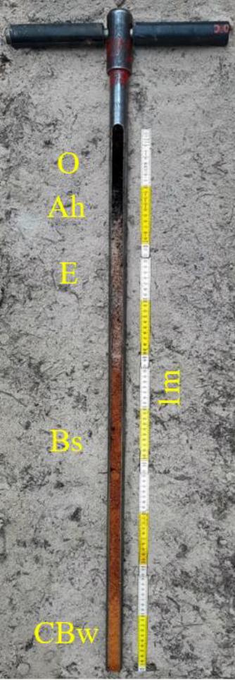
Now place the auger onto the ground. Cut the protruding soil material with a knife and remove it to the side. Avoid contaminating one layer with the removed material from another. Be aware that compaction inside the auger may have occurred; the layer depths may therefore not be accurate. Place a folding ruler aside the auger according to the actually reached depth (Figure 8.2).

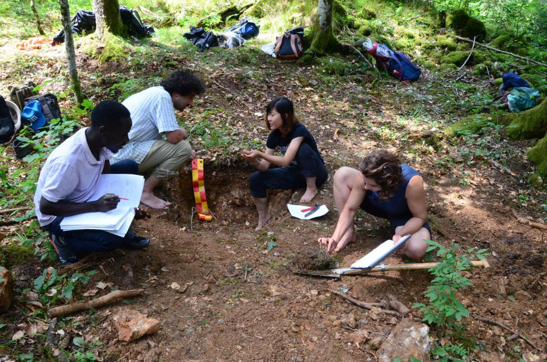
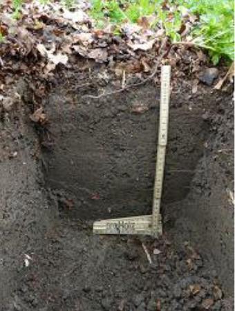
In most cases, the topsoil falls out of the auger. To investigate it in more detail, always make a mini-profile close to where the auger was driven in. It should be at least 25 cm deep and wide, and the profile walls should be vertical and smooth. Now place a folding ruler inside the profile in such a way that point 0 is at the soil surface (see Chapter 8.3.1). For later reconstruction, it may help to take a picture of the mini-profile (Figure 8.3).

The characteristics that can be described from the soil material in the auger are marked with an asterisk (*) in Chapter 8.4.

Figure 8.2: Pürckhauer auger profile

Figure 8.3: Mini-profile

8.1.2 Preparation of a soil profile

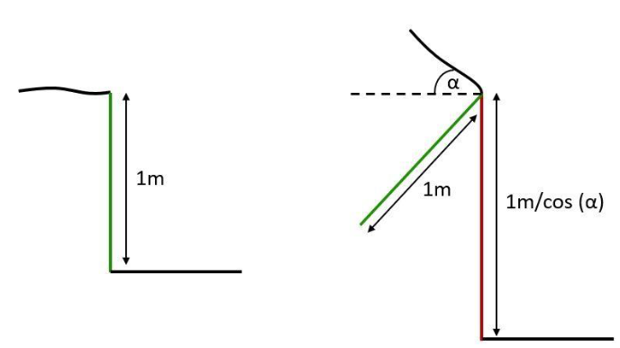
The soil profile should be at least 1 m deep or reach the parent material. On a slope, unless the parent material starts at smaller depth, the profile depth (Figure 8.4) should be 1 m / cos(α). For the decision if the thickness and depth criteria of the WRB are fulfilled and when calculating element stocks (Prietzel and Wiesmeier 2019) the layer thickness perpendicular to the slope is needed. This is calculated multiplying the vertical thickness by cos(α).

Figure 8.4: Correct profile depth when terrain is inclined

The profile should be 1 m wide. If on a slope, the profile wall must be parallel to the contour lines. The material should be piled up to the left and/or right side of the profile and must not be placed on top side of the profile (the side of the profile wall). Never walk or place tools on the side of the profile wall. It is recommended to collect the soil material on two tarps, topsoil and subsoil separately. When refilling the soil profile later, you should first fill in the subsoil and then the topsoil.

Figure 8.5: Ideal soil profile. Always take the photo perpendicular to the profile wall

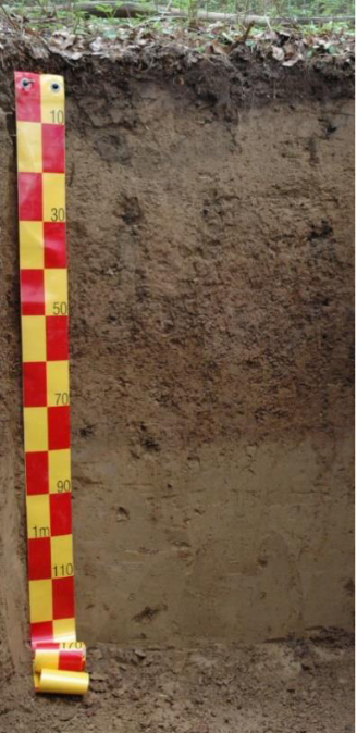
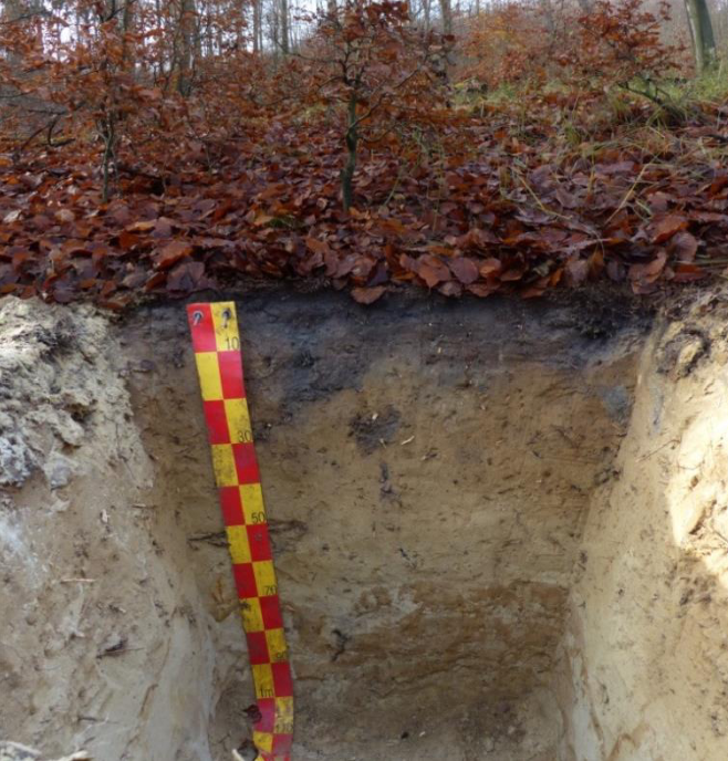
Carefully prepare the profile wall: it must be strictly vertical and smooth. Roots should be cut directly at the profile wall. Use an appropriate tool to clean the profile wall horizontally and avoid vertical smearing. Place the measuring tape in such a way that point 0 is at the soil surface (see Chapter 8.3.1). It should be at one side but not touch the side walls. It must be strictly vertical and plane. It may help to weight the bottom end of the tape with a stone or stick. Take a photo. Hold the camera perpendicularly to the profile wall (Figure 8.5). Avoid any inclination. Also take at least one picture of the surrounding terrain and vegetation (Figure 8.6), e.g., the tree canopy. Make sure you will be able to associate profile and photo later. If possible, save and name the pictures the same day they are taken.

If you describe a soil profile that has been dug some time ago, the topsoil may be disturbed. To describe the humus forms, you need a fresh miniprofile nearby the soil profile.

Figure 8.6: The setting of the profile in the landscape

8.2 General data and description of soil-forming factors

This Chapter refers to some general data and to the soil-forming factors climate, landform and vegetation. Other soil-forming factors are described with the layer description.

8.2.1 Date and authors

Report the date of description and the names of the describing authors.

8.2.2 Location

Give the location a name and report it; e.g., Gombori Pass 1.
Report the GPS coordinates.
Report the altitude above sea level (a.s.l.); e.g., 106 m.

8.2.3 Landform and topography

This Chapter refers to the large-scale topography. For local surface unevenness, see Chapter 8.3.11.

Gradient

Report the ground surface inclination with respect to the horizontal plane. If the profile lies on a flat surface, the gradient is 0%. If it lies on a slope, make 2 records, one upslope and one downslope; e.g., upslope: 18%, downslope: 16%.

Slope aspect

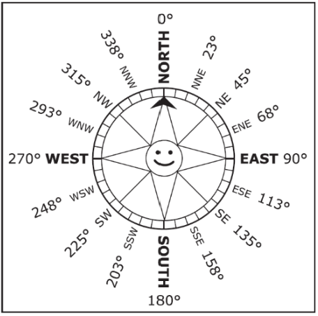
If the profile lies on a slope, report the compass direction that the slope faces, viewed downslope; e.g., 225°.

Figure 8.7: Slope aspect, Schoeneberger et al. (2012), 1-5

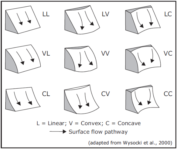
Slope shape

If the profile lies on a slope, report the slope shape in 2 directions: up-/downslope (perpendicular to the elevation contour, i.e. the vertical curvature) and across slope (along the elevation contour, i.e. the horizontal curvature); e.g., Linear, Convex or Concave.

Figure 8.8: Slope Shape, Schoeneberger et al. (2012), 1-6

Position of the soil profile (related to topography)

If the profile lies in an uneven terrain, report the profile position.

Figure 8.9: Position of the profile, Schoeneberger et al. (2012), 1-7, modified (basin not included)

Table 8.1: Position of the profile, Schoeneberger et al. (2012), 1-7, modified

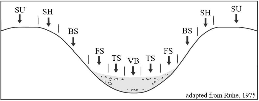
Position	Code
Summit	SU
Shoulder	SH
Backslope	BS
Footslope	FS
Toeslope	TS
Valley bottom	VB
Basin with outflow	OB
Endorheic basin	EB

8.2.4 Climate and weather

Climate

Report the climate according to Köppen (1936) and the ecozones according to Schultz (2005, adapted). The term ‘summer’ refers to the season with high solar altitude and the term ‘winter’ to the season with low solar altitude.

Table 8.2: Climate according to Köppen (1936)

Climate	Code
Tropical climates	A
Tropical rainforest climate	Af
Tropical savannah climate with dry-winter characteristics	Aw
Tropical savannah climate with dry-summer characteristics	As
Tropical monsoon climate	Am
Dry climates	B
Hot arid climate	BWh
Cold arid climate	BWc
Hot semi-arid climate	BSh
Cold semi-arid climate	BSc
Temperate climates	C
Mediterranean hot summer climate	Csa
Mediterranean warm/cool summer climate	Csb
Mediterranean cold summer climate	Csc
Humid subtropical climate	Cfa
Oceanic climate	Cfb
Subpolar oceanic climate	Cfc
Dry-winter humid subtropical climate	Cwa
Dry-winter subtropical highland climate	Cwb
Dry-winter subpolar oceanic climate	Cwc
Continental climates	D
Hot-summer humid continental climate	Dfa
Warm-summer humid continental climate	Dfb
Subarctic climate	Dfc
Extremely cold subarctic climat	Dfd
Monsoon-influenced hot-summer humid continental climate	Dwa
Monsoon-influenced warm-summer humid continental climate	Dwb
Monsoon-influenced subarctic climate	Dwc
Monsoon-influenced extremely cold subarctic climate	Dwd
Mediterranean-influenced hot-summer humid continental climate	Dsa
Mediterranean-influenced warm-summer humid continental climate	Dsb
Mediterranean-influenced subarctic climate	Dsc
Mediterranean-influenced extremely cold subarctic climate	Dsd
Polar and alpine climates	E
Tundra climate	ET
Ice cap climate	EF

Table 8.3: Ecozones according to Schultz (2005, adapted)

Ecozone	Code
Tropics with year-round rain	TYR
Tropics with summer rain	TSR
Dry tropics and subtropics	TSD
Subtropics with year-round rain	SYR
Subtropics with winter rain (Mediterranean climate)	SWR
Humid mid-latitudes	MHU
Dry mid-latitudes	MDR
Boreal zone	BOR
Polar-subpolar zone	POS

Season of Description

Report the season of the description. Vegetation can best be described in the season of full vegetation development.

Table 8.4: Season of description

Ecozone	Season	Code
SYR, SWR, MHU, MDR, BOR, POS	Spring	SP
	Summer	SU
	Autumn	AU
	Winter	WI
TSR	Wet season	WS
	Dry season	DS
TYR, TSD	No significant seasonality for plant growth	NS

Weather conditions

Report the current and past weather conditions.

Table 8.5: Current weather conditions, Schoeneberger et al. (2012), 1-1

Current weather conditions	Code
Sunny/clear	SU
Partly cloudy	PC
Overcast	OV
Rain	RA
Sleet	SL
Snow	SN

Table 8.6: Past weather conditions FAO (2006), Table 2

Past weather conditions	Code
No rain in the last month	NM
No rain in the last week	NW
No rain in the last 24 hours	ND
Rain but no heavy rain in the last 24 hours	RD
Heavy rain for some days or excessive rain in the last 24 hours	RH
Extremely rainy or snow melting	RE

8.2.5 Vegetation and land use

This Chapter refers to all kinds of plant cover from completely natural to completely human-made. It is not a vegetation survey, and only the really soil-relevant characteristics are reported. If the land is cultivated as cropland or grassland, the cultivation type is reported. In all other cases, the vegetation type is reported. Observe an area (10 m x 10 m, if possible) with the profile at its centre.

Vegetation strata

The following strata are relevant.

Table 8.7: Vegetation strata, National Committee on Soil and Terrain (2009), 79, modified

Criterion	Stratum	Code
Ground vegetation	Ground stratum	GS
If both ground stratum and upper stratum are present, you may define a midstratum between the upper stratum and the ground stratum	Mid-stratum	MS
Tallest plants (only if crown cover ≥ 5%)	Upper stratum	ND

Vegetation type or cultivation type

If the land is not cultivated, report the vegetation type according to Table 8.8, for each stratum separately; if more than one type occurs in the same stratum, report up to three, the dominant one first. If the land is cultivated, report the cultivation type according to Table 8.9; cultivated land may show several strata, but they are not reported separately.

Table 8.8: Vegetation strata, National Committee on Soil and Terrain (2009), 79, modified

Life form	Vegetation type	Code
Aquatic	Algae: fresh or brackish	AF
	Algae: marine	AM
	Higher aquatic plants (woody or non-woody)	AH
Surface crusts	Biological crust (of cyanobacteria, algae, fungi, lichens and/or mosses)	CR
Terrestrial non-woody plants	Fungi	NF
	Lichens	NL
	Mosses (non-peat)	NM
	Peat	NP
	Grasses and/or herbs	NG
Terrestrial woody plants	Heath or dwarf shrubs	WH
	Evergreen shrubs	WG
	Seasonally green shrubs	WS
	Evergreen trees (mainly not planted)	WE
	Seasonally green trees (mainly not planted)	WT
	Plantation forest, not in rotation with cropland or grassland	WP
	Plantation forest, in rotation with cropland or grassland	WR
None (barren)	Water, rock, or soil surface with < 0.5% vegetation cover	NO

Table 8.9: Cultivation type

Cultivation type	Code
Simultaneous agroforestry system with trees and perennial crops	ACP
Simultaneous agroforestry system with trees and annual crops	ACA
Simultaneous agroforestry system with trees, perennial and annual crops	ACB
Simultaneous agroforestry system with trees and grassland	AGG
Simultaneous agroforestry system with trees, crops and grassland	ACG
Pasture on (semi-)natural vegetation	GNP
Intensively-managed grassland, pastured	GIP
Intensively-managed grassland, not pastured	GIN
Perennial crop production (e.g. food, fodder, fuel, fiber, ornamental plants)	CPP
Annual crop production (e.g. food, fodder, fuel, fiber, ornamental plants)	CPA
Fallow, less than 12 months, with spontaneous vegetation	FYO
Fallow, at least 12 months, with spontaneous vegetation	FOL
Fallow, all plants constantly removed (dry farming)	FDF

Vegetation height, cover and taxa

For non-cultivated land, report the following characteristics:

• Report the average height and the maximum height in m above ground for each stratum separately.
• Report the vegetation cover. For the upper stratum and the mid-stratum, report the percentage (by area) of the crown cover. For the ground stratum, report the percentage (by area) of the ground cover.
• Report up to three important species per stratum, e.g., Fagus orientalis. If you do not know the species, report the next higher taxonomic rank.

Actual or last cultivated species

For cultivated land, report the actual cultivated species using the scientific name, e.g., Zea mays. If currently under fallow, report the last species and indicate month and year of harvest or of cultivation cessation. If more than one species is/was grown simultaneously, report up to three in the sequence of the area covered, starting with the species that covers the largest area; this includes tree species in simultaneous agroforestry systems.

Rotational cultivated species

For cultivated land, report the species that have been cultivated in the last five years in rotation with the actual or last species. Report up to three in the sequence of frequency, starting with the most frequent species; this includes tree species in rotational agroforestry systems.

Special techniques to enhance site productivity

Report the techniques that refer to the surrounding area of the soil profile. Techniques that affect certain soil layers are reported for the respective layer. Techniques that cause surface unevenness have to be reported in Chapter 8.3.11, additionally. If more than one type is present, report up to three, the dominant one first.

Table 8.10: Special techniques to enhance site productivity

Type	Code
Drainage by open canals	DC
Underground drainage	DU
Wet cultivation	CW
Irrigation	IR
Raised beds	RB
Human-made terraces	HT
Local raise of land surface	LO
Other	OT
None	NO

8.3 Description of surface characteristics

Surface characteristics can be detected on the soil surface without looking into a soil profile.

8.3.1 Soil surface

A litter layer is a loose layer that contains > 90% (by volume, related to the fine earth plus all dead plant residues) recognizable dead plant tissues (e.g. undecomposed leaves). Dead plant material still connected to living plants (e.g. dead parts of Sphagnum mosses) is not regarded to form part of a litter layer. The soil surface (0 cm) is by convention the surface of the soil after removing, if present, the litter layer and, if present, below a layer of living plants (e.g. living mosses). The mineral soil surface is the upper limit of the uppermost mineral horizon (see Chapter 2.1, General rules, and see Chapter 8.4.4).

8.3.2 Litter layer

Observe an area of 5 m x 5 m with the profile at its centre. Report the average and the maximum thickness of the litter layer in cm (see Chapter 8.3.1). If there is no litter layer, report 0 cm as thickness.

8.3.3 Rock outcrops

Rock outcrops are exposures of bedrock. Observe an area (10 m x 10 m if possible) with the profile at its centre. Report the percentage of the area that is covered by rock outcrops. Also report in m the average distance between rock outcrops and their size (average length of the greatest dimension).

8.3.4 Coarse surface fragments

Coarse surface fragments are loose fragments lying at the soil surface, including those partially exposed. Observe an area (5 m x 5 m if possible) with the profile at its centre. The Table indicates the average length of the greatest dimension in cm.

Table 8.11: Size of coarse surface fragments, FAO (2006), Table 15

Size (cm)	Size class	Code
> 0.2 - 0.6	Fine gravel	F
> 0.6 - 2	Medium gravel	M
> 2 - 6	Coarse gravel	C
> 6 - 20	Stones	S
> 20 - 60	Boulders	B
> 60	Large boulders	L
	No coarse surface fragments	N

Report the total percentage of the area that is covered by coarse surface fragments. In addition, report at least one and up to three size classes and report the percentage of the area that is covered by the coarse surface fragments of the respective size class, the dominant one first.

8.3.5 Desert features

Coarse fragments that are constantly exposed to wind-blown sand may be affected by abrasion, etching and polishing, which results in even surfaces with sharp edges. These fragments are called ventifacts (windkanters), and their totality is called desert pavement. Observe an area of 5 m x 5 m with the profile at its centre and report the percentage of ventifacts out of the coarse fragments > 2 cm (greatest dimension).

Coarse fragments may show chemical weathering, which may lead to the formation of oxides and an intense colour at their upper surfaces, whereas there is no such weathering and therefore the original rock colour at their lower surfaces. This intense colour at the upper surfaces is called desert varnish. Observe an area of 5 m x 5 m with the profile at its centre and report the percentage of coarse fragments > 2 cm (greatest dimension) featuring desert varnish.

8.3.6 Patterned ground

Patterned ground is the result of material sorting due to freeze-thaw cycles in permafrost regions. Report the sorting of coarse fragments > 6 cm (greatest dimension) at the soil surface.

Table 8.12: Patterned ground

Form	Code
Rings	R
Polygons	P
Stripes	S
None	N

8.3.7 Surface crusts

Surface crusts are described as layers in Chapter 8.4.31 and further explained there. The area covered is described here. Observe an area (5 m x 5 m if possible) with the profile at its centre. Report the percentage of the area that has a surface crust.

8.3.8 Surface cracks

Cracks are fissures other than those attributed to soil structure (see Chapter 8.4.10). If surface cracks are present, report the average width of the cracks. If the soil surface between cracks of larger width classes is regularly divided by cracks of smaller width classes, report the two width classes. If different width classes occur randomly, just report the dominant one. The continuity of cracks to a greater depth is reported with the layer description (see Chapter 8.4.13). For every width class, report the average distance between the cracks and the spatial arrangement and persistence of the cracks.

Width

Table 8.13: Width of surface cracks, FAO (2006), Table 21

Width (cm)	Width class	Code
≤ 1	Very fine	VF
> 1 - 2	Fine	FI
> 2 - 5	Medium	ME
> 5 - 10	Wide	WI
> 10	Very wide	VW
	No surface cracks	NO

Distance between surface cracks

Table 8.14: Distance between surface cracks, FAO (2006), Table 21, modified

Distance (cm)	Distance class	Code
≤ 0.5	Tiny	TI
> 0.5 - 2	Very small	VS
> 2 - 5	Small	SM
> 5 - 20	Medium	ME
> 20 - 50	Large	LA
> 50 - 200	Very large	VL
> 200 - 500	Huge	HU
> 500	Very huge	VH

Spatial arrangement of surface cracks

Table 8.15: Spatial arrangement of surface cracks

Spatial arrangement	Code
Polygonal	P
Non-polygonal	N

Persistence of surface cracks

Table 8.16: Persistence of surface cracks

Criterion	Code
Reversible (open and close with changing moisture, e.g., in Vertisols and in soils with the Vertic or the Protovertic qualifier)	R
Irreversible (persist year-round, e.g., drained polder cracks, cracks in cemented layers)	I

8.3.9 Presence of water

Report the presence of water above the soil surface. For wet cultivation and irrigation, see Chapter 8.2.5. If water of more than one origin occurs above the soil surface, report the dominant one.

Table 8.17: Water above the soil surface

Criterion	Code
Permanently submerged by seawater (below mean low water springs)	MP
Tidal area (between mean low and mean high water springs)	MT
Occasional storm surges (above mean high water springs)	MO
Permanently submerged by inland water	FP
Submerged by remote flowing inland water at least once a year	FF
Submerged by remote flowing inland water less than once a year	FO
Submerged by rising local groundwater at least once a year	GF
Submerged by rising local groundwater less than once a year	GO
Submerged by local rainwater at least once a year	RF
Submerged by local rainwater less than once a year	RO
Submerged by inland water of unknown origin at least once a year	UF
Submerged by inland water of unknown origin less than once a year	UO
None of the above	NO

8.3.10 Water repellence

Dry soil surfaces may be water-repellent (hydrophobic). Report the water repellence only if the soil surface is dry. Place some water on the soil surface and measure the time until it infiltrates.

Table 8.18: Water repellence

Criterion	Code
Water stands for ≥ 60 seconds	R
Water infiltrates completely within < 60 seconds	N

8.3.11 Surface unevenness

Natural surface unevenness

This paragraph refers to unevenness resulting from soil-forming processes, not associated with erosion, deposition or human activity. Human-made surface unevenness and erosion are reported in the following paragraphs. Deposition is regarded to be a feature of the layers (see Chapter 8.4). Report surface unevenness with an average height difference ≥ 5 cm. Report the type, the average height difference, the average diameter of the elevated areas and the average distance between the height maxima. Give all values in m.

Table 8.19: Types of natural surface unevenness

Criterion	Code
Unevenness caused by permafrost (palsa, pingo, mud boils, thufurs etc.)	P
Unevenness caused by shrink-swell clays (gilgai relief)	G
Other	O
None	N

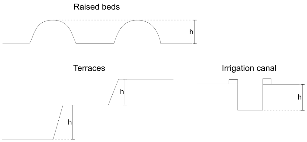
Human-made surface unevenness

Report up to two types of human-made surface unevenness with an average height difference of ≥ 5 cm, the dominant one first. Report only if it shows a repeating pattern. Single characteristics, e.g. a single heap, are not reported. For terraces, report the average height of the terrace wall. For all other features, report the average difference between the highest and the lowest points, the average width/length of the feature, and the average distance between the depth/height maxima. Give all values in cm.

Table 8.20: Types of human-made surface unevenness

Criterion	Code
Human-made terraces	HT
Raised beds	RB
Other longitudinal elevations	EL
Polygonal elevations	EP
Rounded elevations	ER
Drainage canals	CD
Irrigation canals	CI
Other canals	CO
Polygonal holes	HP
Rounded holes	HR
Other	OT
None	NO

Figure 8.10: Human-made surface alterations

Surface unevenness caused by erosion

This paragraph refers to erosion phenomena with an average height difference of ≥ 5 cm. Report category, degree, and activity.

Table 8.21: Categories of erosion, FAO (2006), Table 16

Criterion	Code
Water erosion
Sheet erosion	WS
Rill erosion	WR
Gully erosion	WG
Tunnel erosion	WT
Aeolian (wind) erosion
Shifting sands	AS
Other types of wind erosion	AO
Water and aeolian (wind) erosion	WA
Mass movement (landslides and similar phenomena)	MM
Erosion, not categorized	NC
No evidence of erosion	NO

Table 8.22: Degree of erosion, FAO (2006), Table 18

Criterion	Degree	Code
Some evidence of damage to surface layers, original ecological functions largely intact	Slight	S
Clear evidence of removal of surface layers, original ecological functions partly destroyed	Moderate	M
Surface layers completely removed and subsurface layers exposed, original ecological functions largely destroyed	Severe	V
Substantial removal of deeper subsurface layers, original ecological functions fully destroyed (badlands)	Extreme	E

Table 8.23: Activity of erosion, FAO (2006), Table 19

Criterion	Code
Active at present	PR
Active in recent past (within the last 100 years)	RE
Active in historical times	HI
Period of activity not known	NK

8.3.12 Position of the soil profile (related to surface unevenness)

Report, where the soil profile is located.

Table 8.24: Position of the soil profile, if the soil surface is uneven

Criterion	Code
On the high	H
On the slope	S
In the low	L
On an unaffected surface	E

8.3.13 Technical surface alterations

This Chapter refers to technical surface alterations that do not cause or enhance surface unevenness. For surface unevenness see Chapter 8.3.11. Report the technical surface alterations.

Table 8.25: Technical surface alterations

Criterion	Code
Sealing by concrete	SC
Sealing by asphalt	SA
Other types of sealing	SO
Topsoil removal	TR
Levelling	LV
Other	OT
None	NO

8.4 Description of layers

8.4.1 Identification of layers and layer depths

A soil layer is a zone in the soil, approximately parallel to the soil surface, with properties different from layers above and/or below it. If at least one of these properties is the result of soil-forming processes, the layer is called a soil horizon. In the following, the term ‘layer’ is preferred to include layers, in which soilforming processes did not occur.

A soil layer is identified by certain observable characteristics. Among these characteristics are:

• Matrix colour
• Redoximorphic features
• Texture
• Coarse fragments
• Artefacts
• Bulk density
• Structure
• Coatings and bridges
• Cracks
• Carbonates
• Secondary carbonates
• Secondary gypsum
• Secondary silica
• Cementation
• Water saturation
• Volcanic glasses
• C_org content
• Human alterations

Wherever you observe a major difference in at least one of these characteristics, set a layer boundary. Whenever a layer is too thick (e.g. > 30 cm), it may be wise to subdivide it into two or more layers of more or less equal thickness for description. In certain soils, it may also be wise to add additional layer limits at depths, which you may need to check for the presence or absence of a diagnostic horizon (e.g. 20 cm to check mollic or umbric horizons). Alluvial sediments and tephra layers may be finely stratified. It may be appropriate to combine several such strata to one layer for description. In all other cases, different geological strata must not be combined to one layer.

In the following headings, the (o), the (m), and the (o, m) indicate, whether the described characteristic has to be reported in organic or in mineral layers or in both (see Chapter 8.4.4). For organotechnic layers, the user decides, which characteristics have to be described. The asterisk (*) informs that the characteristic can also be reported in a Pürckhauer auger.

The layers are numbered consecutively from the soil surface (see Chapter 8.3.1) downwards. Report the upper and lower depth for every layer. If the lower depth of the last layer is unknown, report the depth of the profile with the + symbol as the layer’s lower depth.

The following principles have to be considered for description (see General rules, Chapter 2.1):

1. All data refer to the fine earth, unless stated otherwise. The fine earth comprises the soil constituents ≤ 2 mm. The whole soil comprises fine earth, coarse fragments, artefacts, cemented parts, and dead plant residues of any size.
2. All data are given by mass, unless stated otherwise.

8.4.2 Homogeneity of the layer (o, m)

Layer consisting of different parts

If a layer consists of two or more different parts that do not form horizontal layers but can easily be distinguished, describe them separately. Use separate lines in the Soil Description Sheet (Annex 4, Chapter 11) and report the percentage (by exposed area, related to the whole soil) of each part. Examples are layers with retic properties (see Chapter 8.4.18), with cryogenic alteration (see Chapter 8.4.34) or with remodelling by single ploughing (see Chapter 8.4.39). The separation is not recommended, if there is just a wavy boundary (as typical, e.g., for chernic horizons or for eluvial horizons in Podzols, see Chapter 8.4.5) or if there are just some additions of materials (see Chapter 8.4.39).

Layer composed of several strata of alluvial sediments or of tephra

Alluvial strata comprise fluviatile, lacustrine and marine deposits. Tephra strata have a significant amount of pyroclasts. Report the presence of alluvial strata and of tephra strata within the described layer.

Table 8.26: Presence of strata within a layer

Criterion	Code
Layer is composed of two or more alluvial strata	A
Layer is composed of two or more tephra strata	T
Layer is composed of two or more alluvial strata containing tephra	B
Layer is not composed of different strata	N

8.4.3 Water

Water saturation (o, m)

Report the water saturation.

Table 8.27: Types of water saturation

Criterion	Code
Saturated by seawater for ≥ 30 consecutive days	MS
Saturated by seawater according to tidal changes	MT
Saturated by groundwater or flowing water for ≥ 30 consecutive days with water that has an electrical conductivity of ≥ 4 dS m-1	GS
Saturated by groundwater or flowing water for ≥ 30 consecutive days with water that has an electrical conductivity of < 4 dS m-1	GF
Saturated by rainwater for ≥ 30 consecutive days	RA
Saturated by water from melted ice for ≥ 30 consecutive days	MI
Pure water, covered by floating organic material	PW
None of the above	NO

Soil water status (m) (*)

Check the soil water status of non-saturated layers. Spray the profile wall with water and observe the colour change. Then crush a sample and report the behaviour.

Table 8.28: Soil water status, FAO (2006), Table 57, modified

Moistening	Crushing	Moisture class	Code
Going very dark	Dusty or hard	Very dry	VD
Going dark	Makes no dust	Dry	DR
Going slightly dark	Makes no dust	Slightly moist	SM
No change of colour	Makes no dust	Moist	MO
No change of colour	Drops of water	Wet	WE

8.4.4 Organic, organotechnic and mineral layers

We distinguish the following layers (see Chapter 3.3):

• Organic layers consist of organic material.
• Organotechnic layers consist of organotechnic material.
• Mineral layers are all other layers.

An organic or organotechnic layer is called hydromorphic, if water saturation lasts ≥ 30 consecutive days in most years or if it has been drained. Otherwise, it is called terrestrial. Hydromorphic organic layers comprise peat and organic limnic material. Report, whether a layer is organic, organotechnic or mineral and, if organic or organotechnic, whether it is hydromorphic or terrestrial. The distinction is preliminary and may have to be corrected according to laboratory analyses.

Table 8.29: Organic (hydromorphic and terrestrial), organotechnic and mineral layers

Criterion	Code
Organic hydromorphic	OH
Organic terrestrial	OT
Organotechnic hydromorphic	TH
Organotechnic terrestrial	TT
Mineral	MI

8.4.5 Layer boundaries (o, m)

Distinctness of the layer’s lower boundary (*)

Report the distinctness of the layer’s lower boundary.

Table 8.30: Distinctness of layer boundaries, Schoeneberger et al. (2012), 2-6, modified

Mineral layers, organotechnic layers and hydromorphic organic layers: transition within (cm)	Terrestrial organic layers: transition within (cm)	Distinctness	Code
≤ 0.5	≤ 0.1	Very abrupt	V
> 0.5-2	> 0.1-0.2	Abrupt	A
> 2-5	> 0.2-0.5	Clear	C
> 5-15	> 0.5-1	Gradual	G
> 15	> 1	Diffuse	D

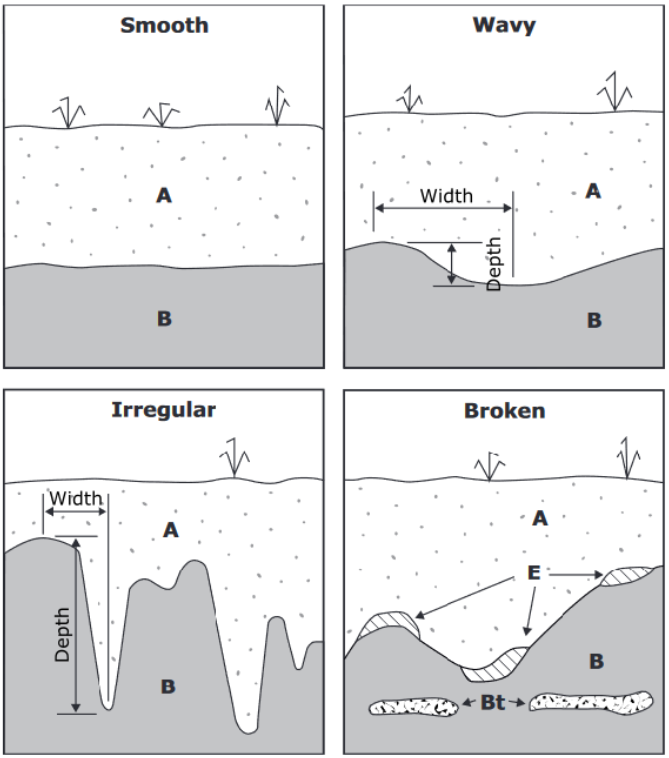
Shape

Report the shape. The characteristic refers to the layer’s lower boundary or, if the shape is ‘broken’, to the entire layer.

Table 8.31: Shape of layer boundaries, Schoeneberger et al. (2012), 2-7

Criterion	Shape	Code
Nearly plane surface	Smooth	S
Pockets less deep than wide	Wavy	W
Pockets more deep than wide	Irregular	I
Discontinuous	Broken	B

Figure 8.11: Shape of layer boundaries, Schoeneberger et al. (2012), 2-7, modified

8.4.6 Wind deposition (m)

Report any evidence of wind deposition. Use a hand lens (maximum 10x).

Table 8.32: Types of wind deposition

Criterion	Code
Aeroturbation (cross-bedding)	CB
≥ 10% of the particles of medium sand or coarser are rounded or subangular and have a matt surface	RH
≥ 10% of the particles of medium sand or coarser are rounded or subangular and have a matt surface, but only in in-blown material that has filled cracks	RC
Other	OT
No evidence of wind deposition	NO

8.4.7 Coarse fragments and remnants of broken-up cemented layers (o, m)

This Chapter refers to natural coarse fragments and to remnants of broken-up cemented layers. Artefacts are described in Chapter 8.4.8. A coarse fragment is a mineral particle, derived from the parent material, > 2 mm in its equivalent diameter (see Chapter 8.4.9). Remnants of broken-up cemented layers may be of any size but are only reported here if they have an equivalent diameter > 2 mm. The subdivisions (0.6 to 60 cm) are according to their greatest dimension.

Size and shape

The Table indicates the length of the greatest dimension and the shape.

Table 8.33: Size and shape classes of coarse fragments and of remnants of broken-up cemented layers, FAO (2006), Tables 27 and 28

Size (cm)	Size Class	Shape	Code
> 0.2-0.6	Fine gravel	Rounded	FR
		Angular	FA
		Rounded and angular	FB
> 0.6-2	Medium gravel	Rounded	MR
		Angular	MA
		Rounded and angular	MB
> 2-6	Coarse gravel	Rounded	CR
		Angular	CA
		Rounded and angular	CB
> 6-20	Stones	Rounded	SR
		Angular	SA
		Rounded and angular	SB
> 20-60	Boulders	Rounded	BR
		Angular	BA
		Rounded and angular	BB
> 60	Large Boulders	Rounded	LR
		Angular	LA
		Rounded and angular	LB
	None		NO

Weathering stage (coarse fragments) and cementing agent (remnants of broken-up cemented layers)

Table 8.34: Weathering stage of coarse fragments, FAO (2006), Table 29

Criterion	Weathering stage	Code
No or little signs of weathering	Fresh	F
Loss of original rock colour and loss of crystal form in the outer parts; centres remain relatively fresh; original strength relatively well preserved	Moderately weathered	M
All but the most resistant minerals weathered; original rock colour lost throughout; tend to disintegrate under only moderate pressure	Strongly weathered	S

Table 8.35: Remnants of broken-up cemented layers: cementing agent

Cementing agent	Code
Secondary carbonates	CA
Secondary gypsum	GY
Secondary silica	SI
Fe oxides, predominantly inside (former) soil aggregates, no significant concentration of organic matter	FI
Fe oxides, predominantly on the surfaces of (former) soil aggregates, no significant concentration of organic matter	FO
Fe oxides, no relationship to (former) soil aggregates, no significant concentration of organic matter	FN
Fe oxides in the presence of a significant concentration of organic matter	FH

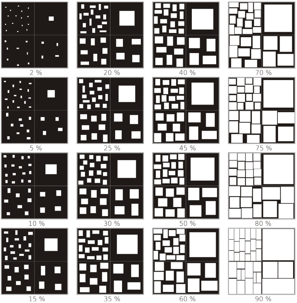
Abundance (by volume)

Report the total percentage of the volume occupied by coarse fragments. In addition, report at least one and up to four size and shape classes and report their weathering stage and the percentage of the volume that is occupied by the coarse fragments of the respective class, the dominant one first. Report the total percentage of the volume occupied by remnants of broken-up cemented layers, report the agent that caused the cementation, where applicable up to two, and the percentage of the volume that is occupied by the remnants of each cementation, the dominant one first (see Chapters 8.4.30 and 8.4.32). All volumes are related to the whole soil. Figure 8.12 helps with the estimation of the volume.

Figure 8.12: Charts for estimating percentages of coarse fragments and of remnants of broken-up cemented layers, FAO , Figure 5, modified by B. Repe

Free large pores (interstices) between coarse fragments

Between coarse fragments, large pores may exist that are visible with the naked eye and do not contain soil material. Report the total percentage (by volume, related to the whole soil).

8.4.8 Artefacts (o, m)

Artefacts are solid or liquid substances that are

• created or substantially modified by humans as part of an industrial or artisanal manufacturing process, or
• brought to the surface by human activity from a depth, where they were not influenced by surface processes, and deposited in an environment, where they do not commonly occur.

Type

Table 8.36: Examples of artefacts, Schoeneberger et al. (2012), 2-50, modified

Type	Code
Bitumen (asphalt), continuous	BT
Bitumen (asphalt), fragments	BF
Black carbon (e.g. charcoal, partly charred particles, soot)	BC
Boiler slag	BS
Bottom ash	BA
Bricks, adobes	BR
Ceramics	CE
Cloth, carpet	CL
Coal combustion byproducts	CU
Concrete, continuous	CR
Concrete, fragments	CF
Crude oil	CO
Debitage (stone tool flakes)	DE
Dressed or crushed stones	DS
Fly ash	FA
Geomembrane, continuous	GM
Geomembrane, fragments	GF
Glass	GL
Gold coins	GC
Household waste (undifferentiated)	HW
Industrial waste	IW
Lumps of applied lime	LL
Metal	ME
Mine spoil	MS
Organic waste	OW
Paper, cardboard	PA
Plasterboard	PB
Plastic	PT
Processed oil products	PO
Rubber (tires etc.)	RU
Treated wood	TW
Other	OT
None	NO

Note: If not purposefully made by humans, black carbon is considered to be natural (see Chapter 8.4.36).

Size

The Table indicates the average length of the greatest dimension of solid artefacts.

Table 8.37: Size of artefacts, FAO (2006), Table 27

Size (cm)	Size class	Code
≤ 0.2	Fine earth	E
> 0.2 - 0.6	Fine gravel	F
> 0.6 - 2	Medium gravel	M
> 2 - 6	Coarse gravel	C
> 6 - 20	Stones	S
> 20 - 60	Boulders	B
> 60	Large boulders	L

Abundance (by volume)

Report the total percentage of the volume (related to the whole soil) occupied by solid artefacts. In addition, report at least one and up to five types and size classes and the percentage of the volume that is occupied by the respective type and size class, the dominant one first. Figure 8.12 helps with the estimation of the volume. Black carbon has to be additionally reported as percentage of the exposed area (related to the fine earth plus black carbon of any size).

8.4.9 Soil texture (m) (*)

Particle-size classes

Table 8.38: Particle-size classes, ISO 11277:2009 (International Organization for Standardization 2015)

Particle-size class	Diameter of particles
Fine earth	all particles ≤ 2 mm
Sand	> 63 μm - ≤ 2 mm
Very coarse sand	> 1250 μm - ≤ 2 mm
Coarse sand	> 630 μm - ≤ 1250 μm
Medium sand	> 200 μm - ≤ 630 μm
Fine sand	> 125 μm - ≤ 200 μm
Very fine sand	> 63 μm - < 125 μm
Silt	> 2 μm - ≤ 63 μm
Clay	≤ 2 μm

The particle size classes up to 2 mm are defined according to the equivalent diameter. The equivalent diameter is the diameter of a sphere that in sedimentation analysis sinks with the same velocity as the respective particle.

The human eye and the tactile sense of the fingers can detect particles > 150-300 μm, depending on individual sensitivity.

Texture classes

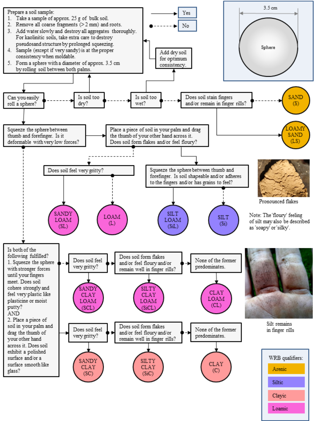
Report the texture class. Please note that the hand-texturing according to the following flow chart only provides an estimation of the texture. Especially around the limits between the classes, the results might be not absolutely reliable. Beginners should ask experienced soil scientists for help.

Figure 8.13: Texture classes, triangle, Blum et al. (2018), Figure 28, modified

Table 8.39: Texture classes, Soil Science Division Staff (2017)

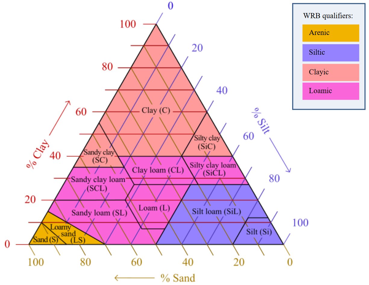
Texture class	% sand	% silt	% clay	Additional criteria
Sand (S)	> 85	< 15	< 10	(%silt + 1.5×%clay) < 15
Loamy sand (LS)	> 70 - ≤ 90	< 30	< 15	(%silt + 1.5×%clay) ≥ 15 and (%silt + 2×%clay) < 30
Silt (Si)	≤ 20	≥ 80	< 12
Silt loam (SiL)	≤ 50	≥ 50 to < 80	< 27
	≤ 8	≥ 80 to ≤ 88	≥ 12 to ≤ 20
Sandy loam (SL)	> 52 - ≤ 85	≤ 48	< 20	(%silt + 2×%clay) ≥ 30
	> 43 - ≤ 52	≥ 41 to < 50	< 7
Loam (L)	> 23 to ≤ 52	≥ 28 to < 50	≥ 7 to < 27
Sandy clay loam (SCL)	> 45 to ≤ 80	< 28	≥ 20 to < 35
Silty clay loam (SiCL)	≤ 20	> 40 to ≤ 73	≥ 27 to < 40
Clay loam (CL)	> 20 to ≤ 45	> 15 to < 53	≥ 27 to < 40
Sandy clay (SC)	> 45 to ≤ 65	< 20	≥ 35 to < 55
Silty clay (SiC)	≤ 20	≥ 40 to ≤ 60	≥ 40 to ≤ 60
Clay (C)	≤ 45	< 40	≥ 40

Figure 8.14: Texture classes, flow chart, ideas adapted from Natural England Technical Information Note TIN037 (2008) and Thien (1979)

Subclasses of the texture classes sand and loamy sand

If the layer belongs to the texture classes sand or loamy sand, report the subclass. The particle-size subclasses of sand are detected by visual estimation of the diameters of the grains or by laboratory analysis. The texture subclasses very fine sand and loamy very fine sand tend to feel floury, whereas all the coarser subclasses feel grainy.

Table 8.40: Subclasses of the texture classes sand and loamy sand, Soil Science Division Staff (2017), modified; the percentages of the sand fractions are related to the entire fine earth (not related to sand).

% very coarse and coarse sand	% medium sand	sum of very coarse, coarse and medium sand	% fine sand	% very fine sand	Feel	Subclasses of the texture class sand	Subclasses of the texture class loamy sand
≥ 25	< 50	Not defined	< 50	< 50	Grainy	Coarse sand (CS)	Loamy coarse sand (LCS)
< 25	Not defined	≥ 25	< 50	< 50	Grainy	Medium sand (MS)	Loamy medium sand (LMS)
≥ 25	≥ 50	Not defined	Not defined	Not defined	Grainy	Medium sand (MS)	Loamy medium sand (LMS)
Not defined	Not defined	Not defined	≥ 50	Not defined	Grainy	Fine sand (FS)	Loamy fine sand (LFS)
Not defined	Not defined	< 25	Not defined	< 50	Grainy	Fine sand (FS)	Loamy fine sand (LFS)
Not defined	Not defined	Not defined	Not defined	≥ 50	Tending to be floury	Very fine sand (VFS)	Loamy very fine sand (LVFS)

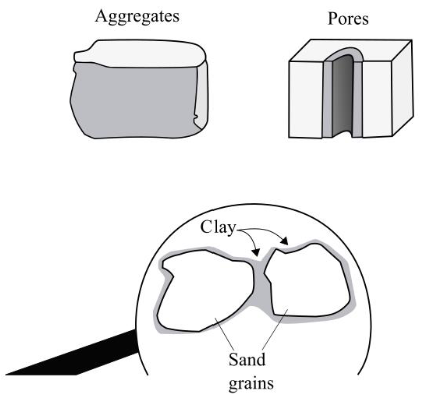
8.4.10 Structure (m)

Structure is the spatial arrangement of soil constituents and pores. If this is, at least partially, the result of soil-forming processes, it is called soil structure. Otherwise, it is rock structure. Structure refers to the fine earth. Structure is reported for mineral layers. Additionally, structure is reported for drained hydromorphic organic layers.

A soil aggregate is a discrete structural body that can be clearly distinguished from its surroundings and that results from soil-forming processes. If a force is applied to a specimen, and the specimen breaks along natural surfaces of weakness, it is composed of aggregates. If the specimen breaks exactly where force is applied, the structure is massive (coherent). If there is no coherence between the particles, the structure is of single-grain type. Human disturbance may create artificial structural elements, which are called clods.

Undisturbed aggregates or non-aggregated structure are called the first-level structure. Aggregates of the types subangular blocky, angular blocky, polyhedral, lenticular, platy, wedge-shaped, prismatic, and columnar may break into aggregates of a second-level structure and even further into aggregates of a third-level structure. The second-level and the third-level structure may be of the same type(s) as the first-level structure or of a different one.

Use the spade, take out a large sample, make sure that the aggregates of the first-level structure, if present, are undisturbed, and observe the structure. Report the type, if present, up to three, the dominant one first. For each type, report separately grade, penetrability for roots, and size class. If applicable, report two size classes, the dominant one first. Report for every type and size class the abundance (as percentage by volume of the layer).

From the first-level structure, take some specimens from each type (if more than one size class of a type is present, take only the greater one) and try to break them with low forces. If aggregates of a second-level structure appear, report the type, if present, up to two, the dominant one first. For each type, report separately grade, size class, and penetrability for roots. If applicable, report two size classes, the dominant one first. Report for every type and size class the abundance (as percentage by volume of the respective first level structure).

From the second-level structure, take some specimens from each type (if more than one size class of a type is present, take only the greater one) and try to break them with low forces. If aggregates of a third-level structure appear, report type, grade, size class, and penetrability for roots. If applicable, report two size classes, the dominant one first. Report for every size class the abundance (as percentage by volume of the respective second level structure).

Types

Figure 8.15 explains some general terms of soil aggregate description.

Figure 8.15: General terms of soil aggregate description

Table 8.41: Types of structure, descriptions, Schoeneberger et al, (2012), 2-53, FAO (2006), Table 49, National Committee on Soil and Terrain (2009), 171-181, modified

Granular		Spheroidal; biogenic; many visible pores; bounded by curved or very irregular faces; limited accommodation to the faces of surrounding aggregates
Subangular blocky		Bounded by undulating rough faces; number of faces variable; many vertices rounded; limited accommodation to the faces of surrounding aggregates
Angular blocky		Bounded by relatively flat smooth, roughly equal faces; number of faces variable; most vertices angular; usually much accommodation to the faces of surrounding aggregates
Lenticular		Bounded by curved faces; overlapping, lens-shaped aggregates generally parallel to the soil surface that are thick at the centre and taper toward the edges; usually much accommodation to the faces of surrounding aggregates; (formed by active or relict frost processes)
Wedge-shaped		Bounded by flat faces; interlocking wedges or lenses that terminate in pronounced angular vertices; ends of vertices may be missing; much accommodation to the faces of surrounding aggregates (typical for first-level or second-level structure in vertic horizons)
Prismatic		Bounded by relatively flat faces; vertically elongated units with angular vertices and flat tops; much accommodation to the faces of surrounding aggregates
Columnar		Bounded by relatively flat faces; vertically elongated units with angular to rounded vertices and rounded (domed) tops
Polyhedral		Bounded by relatively flat smooth, unequal faces; more than six faces; most vertices angular; usually much accommodation to the faces of surrounding aggregates; re-entrant angles between adjoining faces (typical for second-level structure in nitic horizons)
Flat-edged		Bounded by curved faces; lens-shaped aggregates that are thick at the centre and taper toward the edges; limited accommodation to the faces of surrounding aggregates (typical for second-level structure in nitic horizons)
Pseudosand/ Pseudosilt		Spheroidal units of sand and silt size, composed of kaolinite-oxide complexes; the complexes may be interconnected to each other; hand-texturing according to Chapter 8.4.9 first yields the impression of a dominance of sand and silt and after prolonged squeezing proves the dominance of clay
Platy		Bounded by relatively flat horizontal faces; much accommodation to the faces of surrounding aggregates
Single grain		Entirely non-coherent, e.g., loose sand
Massive		Material is a coherent mass (not necessarily cemented)
Cloddy		Artificial clods created by disturbance; e.g., ploughing

Table 8.42: Types of structure, formation and codes

Type	Formation	Code
Granular	Soil aggregate structure, natural	GR
Subangular blocky	Soil aggregate structure, natural	BS
Angular blocky	Soil aggregate structure, natural	BA
Lenticular	Soil aggregate structure, natural	LC
Wedge-shaped	Soil aggregate structure, natural	WE
Prismatic	Soil aggregate structure, natural	PR
Columnar	Soil aggregate structure, natural	CO
Polyhedral	Soil aggregate structure, natural	PH
Flatedged	Soil aggregate structure, natural	FE
Pseudosand/ Pseudosilt	Soil aggregate structure, natural	PS
Platy	Soil aggregate structure, natural or resulting from artificial pressure	PL
Single grain	No structural units, rock structure, inherited from the parent material	SR
Single grain	No structural units, soil structure, resulting from soil-forming processes, like loss of organic matter and/or oxides and/or clay minerals or loss of stratification	SS
Massive	No structural units, rock structure, inherited from the parent material, structure not changing with soil moisture, not or only slightly chemically weathered	MR
Massive	No structural units, rock structure, inherited from the parent material, structure not changing with soil moisture, strongly chemically weathered (e.g. saprolite)	MW
Massive	No structural units, soil structure, present when moist and changing into soil aggregate structure when dry	MS
Stratified	No structural units, rock structure, visible stratification from sedimentation	ST
Cloddy	Artificial structural elements	CL

Grade

Table 8.43: Grade of structural units, Soil Science Division Staff (2017), 159f, modified

Criterion	Grade	Code
The units are barely observable in place. When gently disturbed, the soil material parts into a mixture of whole and broken units, the majority of which exhibit no surfaces of weakness. The surfaces differ in some way from the interiors.	Weak	W
The units are well formed and evident in place. When disturbed, the soil material parts into a mixture of mostly whole units, some broken units, and material that is not in units. Aggregates part from adjoining aggregates to reveal nearly entire faces that have properties distinct from those of fractured surfaces	Moderate	M
The units are distinct in place. When disturbed, they separate cleanly, mainly into whole units. Aggregates have distinct surface properties.	Strong	S

Penetrability for roots

Large soil aggregates may have a dense outer rim that does not allow roots to enter.

Table 8.44: Aggregate penetrability for roots

Criterion	Code
All aggregates with dense outer rim	P
Some aggregates with dense outer rim	S
No aggregate with dense outer rim	N

Size

The dimension to be reported is indicated in Table 8.41 by a line.

Table 8.45: Aggregate size, Schoeneberger et al. (2012), 2-55, FAO (2006), Table 50, modified

Criterion: size of structural unit (mm)			Size Class	Code
Granular, Flat-edged, Platy	Subangular blocky, Angular blocky, Lenticular, Polyhedral, Cloddy	Wedge-shaped, Prismatic, Columnar
≤ 1	≤ 5	≤ 10	Very fine	VF
> 1-2	> 5-10	> 10-20	Fine	FI
> 2-5	> 10-20	> 20-50	Medium	ME
> 5-10	> 20-50	> 50-100	Coarse	CO
> 10-20	> 50-100	> 100-300	Very coarse	VC
> 20	> 100	> 300	Extremely coarse	EC

Inclination of wedge-shaped aggregates

If wedge-shaped aggregates are present, report the volume (as percentage), occupied by wedge-shaped aggregates tilted between ≥ 10° and ≤ 60° from the horizontal.

8.4.11 Pores and cracks (overview)

Soil has air- or water-filled voids, which are:

• Interstitial (primary packing voids)
• Non-matrix pores (tubular, dendritic tubular, vesicular, irregular)
• Interstructural (fractures between soil aggregates, which can be inferred from soil structure description)
• Cracks (fissures other than those attributed to soil structure). We only report non-matrix pores and cracks.

8.4.12 Non-matrix pores (m)

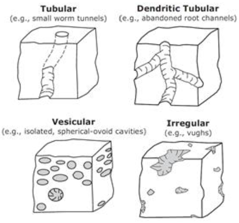
Type

Table 8.46: Types of non-matrix pores, Schoeneberger et al. (2012), 2-73, modified

Criterion	Type	Code
Cylindrical and elongated voids; e.g., worm tunnels	Tubular	TU
Cylindrical, elongated, branching voids; e.g., empty root channels	Dedritic Tubular	DT
Ovoid to spherical voids; e.g., solidified pseudomorphs of entrapped gas bubbles concentrated below a crust; most common in arid and semiarid environments and in permafrost soils	Vesicular	VE
Non-connected cavities, chambers; e.g., vughs; various shapes	Irregular	IG
No non-matrix pore		NO

Tubular and dendritic tubular pores are commonly referred to as biopores.

Figure 8.16: Type of non-matrix pores, Schoeneberger et al. (2012), 2-74

Size and abundance

Table 8.47: Pore size, Schoeneberger et al. (2012), 2-70

Diameter (mm)	Soil area to be assessed	Size Class	Code
≤ 1	1 cm2	Very Fine	VF
> 2-5	1 cm2	Fine	FI
> 5-10	1 dm2	Medium	ME
> 5-10	1 dm2	Coarse	CO
> 10	1 m2	Very coarse	VC

Table 8.48: Abundance of pores, Schoeneberger et al. (2012), 2-70, modified

Number	Abundance class	Code
≤ 1	Very few	V
> 1-3	Few	F
> 3-5	Common	C
> 5	May	M

Report all non-matrix pore types that apply. For every type and every size class, count the number of pores in the assessed area. For every type, report the dominant size class (size class that has the highest number of pores). For every type, calculate the sum of pores across the size classes and report the abundance class.

Example:

Very fine: 0
Fine: 2
Medium: 2
Coarse: 1
Very coarse: 0

The sum is 5, and the abundance class is Common.

8.4.13 Cracks (o, m)

Report persistence and continuity,

Persistence

Table 8.49: Persistence of cracks, Schoeneberger et al. (2012), 2-76

Criterion	Code
Reversible (open and close with changing soil moisture)	RT
Irreversible (persist year-round)	IT
No cracks	NO

Continuity

Table 8.50: Continuity of cracks

Criterion	Code
All cracks continue into the underlying layer	AC
At least half, but not all of the cracks continue into the underlying layer	HC
At least one, but less than half of the cracks continue into the underlying layer	SC
Cracks do not continue into the underlying layer	NC

Width and abundance

Report the average width in mm and the number of cracks. Count the cracks across 1 m horizontally; use the vertical centre of the layer.

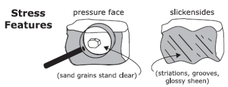
8.4.14 Stress features (m)

Stress features result from soil aggregates that are pressed against each other due to swelling clays. The aggregate surfaces may be shiny. There are two types: Pressure faces do not slide past each other and have no striations, slickensides slide past each other and have striations. Striations develop if sand (or silt) grains are moved with strong pressure along the aggregate surfaces. Stress features do not differ in colour from the matrix (see Chapter 8.4.17). A hand lens (maximum 10x) may be helpful. Report the abundance of

• Pressure faces in % of the surfaces of soil aggregates
• Slickensides in % of the surfaces of soil aggregates.

{#fig-a1-817}

8.4.15 Concentrations (overview)

The following definitions apply to concentrations, e.g., redox concentrations or secondary carbonates (some concentrations may not show all the below-listed types). For cementation classes, see Chapter 8.4.30.

Table 8.51: Types of concentrations (overview), Soil Science Division Staff. (2017), page 174f

Description	Designation
Rounded body, at least very weakly cemented, that can be removed as discrete unit, with internal organization in the form of concentric layers that are visible to the naked eye	Concretion
Rounded body, at least very weakly cemented, that can be removed as discrete unit, without evident internal organization	Nodule
Longitudinal body of any cementation class	Filament
Non-cemented or extremely weakly cemented body, of various shape, that cannot be removed as discrete unit	Mass

8.4.16 Soil colour (overview)

In general, soil colour can be a property of the four following soil features:

• Matrix (see Chapter 8.4.17 and Chapter 8.4.18)
• Lithogenic variegates (see Chapter 8.4.19)
• Redoximorphic features, resulting from redox processes (see Chapter 8.4.20)
• Non-redoximorphic features, resulting from other pedogenic processes:
  • initial weathering (see Chapter 8.4.22)
  • clay coatings and bridges (see Chapter 8.4.23)
  • uncoated sand and/or coarse silt grains (see Chapter 8.4.23)
  • ribbon-like accumulations (see Chapter 8.4.24)
  • secondary carbonates (see Chapter 8.4.25)
  • secondary gypsum (see Chapter 8.4.26)
  • secondary silica (see Chapter 8.4.27)
  • readily soluble salts (see Chapter 8.4.28)
  • accumulations of organic matter (see Chapter 8.4.36)

%%{ init: { 'flowchart': { 'curve': 'stepAfter' } } }%%
flowchart TD
  St[Colour]-->q1{Is the colour \n a matrix colour?}
  %% TODO fix rendering of yes/no answers to have a halo etc - bug?
  q1 -->|Yes|r1["Matrix colour(s)"]
  q1 -.->|No|q2{Is the colour \n the result of \npedogenic processes?}
  q2 -.->|No|r2[Lithogenic mottle]
  q2 -->|Yes|q3{Are the features \n formed by redox \nprocesses?}
  q3 -->|Yes|r3[Redoximorphic features]
  q3 -.->|No|r4[Non-redoximorphic features]

Figure 8.17: Colour flow chart, Schoeneberger et al. (2012), 2-8, modified

Use the Munsell Color Charts. Take a fresh sample, slightly crush it and observe the colour in the shade (both your eyes and the colour chart in the shade) and not in the twilight. Report hue, value and chroma. The matrix colour and the colour of reductimorphic features are recorded twice, moist and (if possible) dry, the other colours only in the moist state. The moist state corresponds to field capacity, which is obtained with sufficient accuracy by moistening and reading the colour as soon as visible moisture films have disappeared.

8.4.17 Matrix colour (m) (*)

Report the colour of the soil matrix. If there is more than one matrix colour, report up to three, the dominant one first, and give the percentage of the exposed area.

Advanced chemical weathering without physical alteration, especially without turbation, results in saprolite (see Chapter 8.4.10). According to the minerals present, a colour pattern may result. These colours are reported as matrix colours.

8.4.18 Combinations of darker-coloured finer-textured and lighter-coloured coarser-textured parts (m)

If a layer consists of darker-coloured finer-textured and lighter-coloured coarser-textured parts that do not form horizontal layers but can easily be distinguished, describe them separately. Use separate lines in the Soil Description Sheet (Annex 4, Chapter 11) and give a full description. The principal colours are regarded to be matrix colours.

For the coarser-textured parts, report in addition the following characteristics:

• the percentage (by exposed area) occupied by coarser-textured parts of any orientation (vertical, horizontal, inclined) having a width of ≥ 0.5 cm
• the percentage (by exposed area) occupied by continuous vertical tongues of coarser-textured parts with a horizontal extension of ≥ 1 cm (if these tongues are absent, report 0%)
• the depth range in cm, where these tongues cover ≥ 10% of the exposed area (if they extend across serveral layers, the length is only reported in the description of that layer, where they start at the layer’s upper limit).

In the middle of the layer, prepare a horizontal surface, 50 cm x 50 cm, and report the percentage (by horizontal area covered) of the coarser-textured parts.

8.4.19 Lithogenic variegates (m)

Report colour, size class, and abundance. If more than one colour occurs, report up to three, the dominant one first, and give size class and abundance for each colour separately.

Colour

Report the colour according to the Munsell Color Charts. Write ‘None’ if there are no lithogenic variegates.

Size

The Table indicates the average length of the greatest dimension.

Table 8.52: Size of lithogenic variegates, FAO (2006), Table 33

Size (mm)	Size class	Designation
≤ 2	Very fine	V
> 2-6	Fine	F
> 6-20	Medium	M
> 20	Coarse	C

Abundance (by exposed area)

Report the percentage of abundance.

8.4.20 Redoximorphic features (m)

Redoximorphic features (oximorphic features plus reductimorphic features) are the result of redox processes. Oximorphic features show the accumulation of substances in oxidized state and usually a redder hue, a higher chroma and a lower value than the surrounding material, while reductimorphic features show the opposite characteristics. Soil parts showing reductimorphic features may either contain substances in reduced state or may have lost them.

Report substance, location, size class (up to two, the dominant one first), cementation class and abundance for each colour separately, for up to three colours, the dominant one first. Substance for oximorphic features is always reported, for reductimorphic features only in some cases. Size class is only reported for oximorphic features inside soil aggregates. Cementation is only reported for oximorphic features. The abundance is reported as percentage of the exposed area.

Colour (*)

Report the colour according to the Munsell Color Charts. Write ‘None’ if there are no redoximorphic features.

Substance (*)

Table 8.53: Substance of oximorphic features

Substance	Code
Fe oxides	FE
Mn oxides	MN
Fe and Mn oxides	FM
Jarosite	JA
Schwertmannite	SM
Fe and Al sulfates (not specified)	AS

The term ‘oxides’, as used here, includes hydroxides and oxide-hydroxides. The term ‘sulfates’ includes hydroxysulfates.

Table 8.54: Substance of reductimorphic features

Substance	Code
Fe sulfides	FS
No visible accumulation	NV

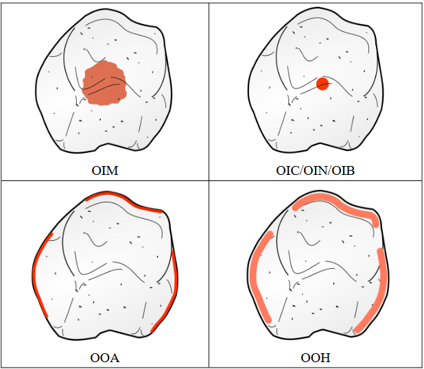
Location (*)

Table 8.55: Location of some reductimorphic features

Location		Code
Inner parts	Inside soil aggregates: masses	OIM
	Inside soil aggregates: concretions	OIC
	Inside soil aggregates: nodules	OIN
	Inside soil aggregates: both concretions and/or nodules (not possible to distinguish)	OIB
Outer parts	On surfaces of soil aggregates	OOA
	Adjacent to surfaces of soil aggregates, infused into the matrix (hypocoats)	OOH
	On biopore walls, lining the entire wall surface	OOE
	On biopore walls, not lining the entire wall surface	OON
	Adjacent to biopores, infused into the matrix (hypocoats)	OOI
Random (not associated with aggregate surfaces or pores)	Distributed over the layer, no order visible	ORN
	Distributed over the layer, surrounding areas with reductimorphic features	ORS
	Throughout	ORT

Figure 8.18: Location of some oximorphic features

Table 8.56: Location of reductimorphic features

Location		Code
Inner parts	Inside soil aggregates	RIA
Outer parts	Outer parts of soil aggregates	ROA
	Around biopores, surrounding the entire pores	ROE
	Around biopores, not surrounding the entire pores	RON
Random (not associated with aggregate surfaces or pores)	Distributed over the layer, no order visible	RRN
	Distributed over the layer, surrounding areas with oximorphic features	RRS
	Throughout	RRT

Size of oximorphic features (*)

The Table indicates the average length of the greatest dimension.

Table 8.57: Size of oximorphic features, FAO (2006), Table 33

Size (mm)	Size Class	Code
≤ 2	Very fine	VF
> 2 - 6	Fine	FI
> 6 - 20	Medium	ME
> 20 - 60	Coarse	CO
> 60	Very coarse	VC

Cementation class of oximorphic features (*)

If an intact specimen is not obtainable, the oximorphic feature is not cemented. Otherwise, take out the feature, apply force perpendicular to its greatest dimension, observe the force needed for failure and report the cementation class.

Table 8.58: Consistence of oximorphic features, Schoeneberger et al. (2012), 2-63

Criterion	Class	Code
Intact specimen not obtainable or very slight force between fingers, < 8 N	Not cemented	NC
Slight force between fingers, 8 - < 20 N	Extremely weakly cemented	EWC
Moderate force between fingers, 20 - < 40 N	Very weakly cemented	VWC
Strong force between fingers, 40 - < 80 N	Weakly cemented	WEC
Does not fail when applying force between fingers, ≥ 80 N	Moderately or more cemented	MOC

Abundance (by exposed area)

Report the total abundance of the parts with oximorphic features and the total abundance of the parts with reductimorphic features, both for inner, outer and random locations, separately. Report them as percentage of the exposed area (related to the fine earth plus oximorphic features of any size and any cementation class).

Abundance of cemented oximorphic features (by volume, related to the whole soil)

This paragraph refers to cemented oximorphic features with a cementation class of at least moderately cemented and a diameter of > 2 mm. They comprise concretions and nodules (see above) and remnants of a broken-up layer that has been cemented by Fe oxides. Report the abundance as percentage by volume (related to the whole soil).

8.4.21 Redox potential and reducing conditions (o, m)

The soil redox potential (Eh) expresses the ratio of the concentrations of oxidized and reduced substances and is measured in millivolts (mV). In soils, redox potentials range from +800 mV to –350 mV. A low redox potential indicates strong reducing conditions. When opening a profile pit, oxygen gets access to the profile wall, which leads to a rapid oxidation of the exposed reduced substances and to a subsequent change of the redox potential at the profile wall.

Measure the redox potential and calculate the rH value

For measuring the redox potential (Blume, Stahr, and Leinweber 2010; UN-FAO 2006), the following equipment is needed:

• a pointed stainless-steel rod of 4-5 mm in diameter, long enough to reach the desired soil depth
• a perforated plastic tube of 15-20 mm in diameter and of a length corresponding to the depth of measurement
• concentrated KCl solution, fixed with agar
• a Pt electrode
• a reference electrode, e.g., with Ag/AgCl in 1 M KCl or with calomel (as used for measuring the pH value)
• a potentiometer.

Procedure: Step 1 - 2 m aside the profile pit and drive the rod into the soil down to the desired depth, roughen the Pt electrode with fine-grained sandpaper, intrude it immediately into the hole and press it against the soil. Make another hole at 10-20 cm distance, wide and deep enough to place a plastic tube that is some cm longer than the depth of the Pt electrode. Fill the tube with the fixed KCl solution, place the tube into the hole and fix it with soil material. Then, place the reference electrode into the KCl solution. Connect the electrodes with the potentiometer and read the voltage after 30 minutes. Repeat readings every 10 minutes until the value is stable. In some cases, this may take several hours. At least two replicates are recommended. (If you dispose of more than one set of equipment, you may measure the redox potential simultaneously at different soil depths.) The obtained voltage has to be adjusted to the voltage of the standard hydrogen electrode: for Ag/AgCl in 1 M KCl add +244 mV, for calomel add +287 mV. Simultaneously, measure the pH value (see Chapter 8.4.29) of the soil at the profile wall in distilled water (soil:water = 1:5) at the same depth. Report the rH value that is calculated with the following equation: \(rH = (2 Eh \div 59) + 2 pH\)

Note: If the profile is freshly dug and not too sandy, you may also place the electrodes horizontally at least 15 cm behind in the profile wall.

Estimate the rH value (*)

The following field tests are available to prove reducing conditions:

• Methane can be lit with a match.
• H₂S is formed when spraying a soil sample with a 10% HCl solution and can be identified by the odour of rotten eggs.
• Fe²⁺ can be proven by oxidation with a 0.2% (mass by volume) solution of α,α-dipyridyl dissolved in 1 N ammonium acetate (NH₄OAc), pH 7. Take a soil sample and spray it with the solution. If Fe²⁺ is present, a strong red colour will develop. The test needs a freshly broken sample that has not yet been oxidized at the open profile wall. In neutral to alkaline soils, the colour is hardly visible. Caution: The solution is slightly toxic.

The following Table explains how to estimate the rH value using these field tests and the observed redoximorphic features (see Chapter 8.4.20). Report the rH range. Note that oximorphic features may be relic. Reductimorphic features may also be relic, if Fe and Mn have been removed in reduced form leaving behind a layer virtually free of Fe and Mn.

Table 8.59: Ranges of rH values and related soil processes as derived from redoximorphic features and from field tests of reducing conditions, Blume et al. (2010), page 24, FAO (2006), Table 36, modified

Criterion	Processes	rH value (V)	Code
No redoximorphic features	Strongly aerated	> 33	R6
	Denitrification	29 - 33	R6
Oximorphic features of Mn; temporally no free oxygen present	Redox reactions of Mn	temporally 20 - 29	R5
Oximorphic features of Fe	Redox reactions of Fe	temporally < 20	R4
Blue-green to grey colour, Fe2 ions always present (reduced areas show a positive α,α-dipyridyl test)	Formation of Fe2/Fe3 oxides (green rust)	13 - 20	R3
Black colour due to metal sulfides (spraying with a 10% HCl solution causes the formation of H2S)	Sulfide formation	10 - 13	R2
Flammable methane present	Methane formation	< 10	R1

8.4.22 Initial weathering (m)

A major process of chemical weathering is the formation of Fe oxides (including hydroxides and oxide-hydroxides). If the weathering is initial, the Fe oxides may be concentrated in soil parts with easy access to oxygen, e.g. along pores. These parts have a distinctly redder hue or stronger chroma. Report the abundance as percentage of the exposed area.

8.4.23 Coatings and bridges (m)

Clay coatings and clay bridges

Illuviated clay consists of clay minerals, mostly together with oxides and in many cases together with organic matter. It covers surfaces of soil aggregates, coarse fragments and biopore walls as coatings (argillans), or it forms bridges between sand grains. The clay minerals give the coatings a shiny appearance. The oxides provide a colour that is more intensive (usually a higher Munsell chroma) than the colour of the matrix; organic matter provides a darker colour (usually a lower Munsell value) than the colour of the matrix (see Chapter 8.4.17). A hand lens (maximum 10x) may be helpful.

Report the abundance of

• clay coatings in % of the surfaces of soil aggregates, coarse fragments and/or biopore walls
• clay bridges between sand grains in % of involved sand grains.

Figure 8.19: Clay coatings and clay bridges, Schoeneberger et al. , 2-34

Organic matter coatings and oxide coatings on sand and coarse silt grains

Sand and coarse silt grains are mostly coated by organic matter and/or oxides. In certain layers, these coatings may be cracked. In other layers, these coatings may be missing.

Table 8.60: Organic matter coatings and oxide coatings on sand and/or coarse silt grains

Criterion	Code
Cracked coatings on sand grains	C
Uncoated sand and/or coarse silt grains	U
All sand and coarse silt grains coated without cracks	A

For C, report the percentage related to the estimated number of sand grains. For U, report the percentage related to the estimated number of sand and coarse silt grains.

8.4.24 Ribbon-like accumulations (m) (*)

Ribbon-like accumulations are thin, horizontally continuous accumulations within the matrix of another layer. Report the accumulated substance(s).

Table 8.61: Substances of ribbon-like accumulations

Criterion	Code
Clay minerals	CC
Fe oxides and/or Mn oxides	OO
Organic matter	HH
Clay minerals and Fe oxides and/or Mn oxides	CO
Clay minerals and organic matter	CH
Fe oxides and/or Mn oxides and organic matter	OH
Clay minerals, Fe oxides and/or Mn oxides and organic matter	TO
No ribbon-like accumulations	NO

The term ‘oxides’, as used here, includes hydroxides and oxide-hydroxides. If clay minerals are accumulated, a ribbon-like accumulation is < 7.5 cm thick, in all other cases < 2.5 cm. If there are 2 or more ribbon-like accumulations in one layer, report the number of the accumulations and their combined thickness in cm. If clay minerals are accumulated (CC, CO, CH, TO), the ribbon-like accumulations are called lamellae.

8.4.25 Carbonates (o, m)

Take a soil sample, add drops of 1 M HCl and observe the reaction. This method detects primary and secondary calcium carbonates. Contrary to calcium carbonate, dolomite (calcium magnesium carbonate) shows little reaction with cold HCl. To identity dolomite, put some soil material in a spoon, add drops of 1 M HCl and heat it with a lighter underneath. If effervescence occurs only after heating, the presence of dolomite is indicated.

Content (*)

Report the carbonate content in the soil matrix and report, whether the reaction with HCl is immediate or only after heating.

Table 8.62: Carbonate contents, FAO (2006), Table 38

Criterion	Content	% (by mass)	Code
No visible or audible effervescence	Non-calcareous	0	NC
Audible effervescence but not visible	Slightly calcareous	> 0 - 2	SL
Visible effervescence	Moderately calcareous	> 2 - 10	MO
Strong visible effervescence, bubbles form a low foam	Strongly calcareous	> 10 - 25	ST
Extremely strong reaction, thick foam forms quickly	Extremely calcareous	> 25	EX

Table 8.63: Retarded reaction with HCl

Criterion	Code
Reaction with 1 M HCl immediate	I
Reaction with 1 M HCl only after heating	H

Secondary carbonates

Report the type of secondary carbonates. If more than one occurs, report up to four, the dominant one first. Report secondary carbonates only if visible when moist. Always check with HCl if it is really carbonate. Report the abundance as percentage for each form using Table 8.65 as a reference.

Table 8.64: Types of secondary carbonates

Type	Code
Masses (including spheroidal aggregations like white eyes (byeloglaska))	MA
Nodules and/or concretions	NC
Filaments (including continuous filaments like pseudomycelia)	FI
Coatings on soil aggregate surfaces or biopore walls	AS
Coatings on undersides of coarse fragments and of remnants of broken-up cemented layers	UR
No secondary carbonates	NO

Table 8.65: Reference for estimating the percentage of secondary carbonates

Code	Reference for estimating the percentage
MA, NC, FI	Exposed area (related to the fine earth plus accumulations of secondary carbonates of any size and any cementation class)
AS	Soil aggregate and biopore wall surfaces
UR	Underside surfaces

8.4.26 Gypsum (m)

Content

Report the gypsum content in the soil matrix. If readily soluble salts are absent or present in small amounts only, gypsum can be estimated by measuring the electrical conductivity in soil suspensions of different soil-water relations after 30 minutes (in the case of fine-grained gypsum). This method detects primary and secondary gypsum. Note: Higher gypsum contents may be differentiated by abundance of H₂O-soluble pseudomycelia/crystals and a soil colour with high value and low chroma.

Table 8.66: Gypsum contents in layers with little readily soluble salts, FAO (2006), Table 40

Electrical conductivity (EC)	Content	% (by mass)	Code
≤ 1.8 dS m-1 in 10 g soil / 25 ml H2O or ≤ 0.18 dS m-1 in 10 g soil / 250 ml H2O	Non-gypsiferous	0	NG
> 0.18 - ≤ 1.8 dS m-1 in 10 g soil / 250 ml H2O	Slightly gypsiferous	> 0 - 5	SL
> 1.8 dS m-1 in 10 g soil / 250 ml H2O	Moderately gypsiferous	> 5 - 15	MO
> 1.8 dS m-1 in 10 g soil / 250 ml H2O	Strongly gypsiferous	> 15 - 60	ST
> 1.8 dS m-1 in 10 g soil / 250 ml H2O	Extremely gypsiferous	> 60	EX

Secondary gypsum

Secondary gypsum may be found as

• filaments (vermiform gypsum, pseudomycelia)
• gypsum crystal intergrowths or nodules (roses)
• pendants (normally fibrous) below coarse fragments and below remnants of broken-up cemented layers
• fibrous aggregates
• flour-like gypsum.

Gypsum is soft and can easily be ripped with a knife or broken between thumbnail and forefinger. Gypsum is very soluble, and when gypsum is found in soils that are not in extremely arid conditions, it can be assumed that it is secondary in almost all cases. Contrary to that, gypsiferous rocks and their fragments are primary. Fibrous gypsum, when occurring along veins within limestones or sandstones is also primary. Report the total abundance (as percentage by exposed area, related to the fine earth plus accumulations of secondary gypsum of any size and any cementation class) of all types of secondary gypsum.

8.4.27 Secondary silica (m)

Form

Secondary silica (SiO₂) is off-white and predominantly consisting of opal and microcrystalline forms. It occurs as laminar caps, lenses, (partly) filled interstices, bridges between sand grains, and as coatings at surfaces of soil aggregates, biopore walls, coarse fragments, and remnants of broken-up cemented layers. Report the type of secondary silica. If more than one type occurs, report up to two, the dominant one first. Note: Durinodes are often coated with secondary carbonates.

Table 8.67: Types of secondary silica

Type	Code
Nodules (durinodes)	DN
Accumulations within a layer, cemented by secondary silica	CH
Remnants of a layer that has been cemented by secondary silica	FC
Other accumulations	OT
No secondary silica	NO

Size

If a layer shows durinodes and/or remnants of a layer that has been cemented by secondary silica, report their size class. The Table indicates the average length of the greatest dimension.

Table 8.68: Size of durinodes and remnants of a layer that has been cemented by secondary silica

Size (cm)	Size class	Code
≤ 0.5	Very fine	VF
> 0.5 - 1	Fine	FI
> 1 - 2	Medium	ME
> 2 - 6	Coarse	CO
> 6	Very coarse	VC

Abundance

Report the total percentage (by exposed area) of secondary silica. For a cemented layer, this percentage refers to the fine earth plus accumulations of secondary silica of any size and any cementation class. For durinodes and remnants of a cemented layer, this percentage comprises the secondary silica visible at their surfaces. If a layer shows durinodes and/or remnants of a cemented layer, report in addition the percentage (by volume) of those durinodes and remnants that have a diameter ≥ 1 cm.

8.4.28 Readily soluble salts (o, m)

Readily soluble salts are precipitated in dry soil and dissolved in moist soil. They are more soluble than gypsum. The presence of readily soluble salts is checked by measuring the electrical conductivity in the saturation extract (EC_SE). In the saturation extract, the soil is completely moist, but has no visible water surplus. This is not easy to achieve.

Alternatively, one can measure the electrical conductivity in an extract of 10 g soil with 25 ml aqua dest. (EC_2.5). Mix soil and water carefully, let it rest for at least 30 minutes and measure the electrical conductivity in the clear solution in dS m^-1. It must then be transformed into the EC_SE according to the following equation: \(EC_{SE} = 250 \times EC_{2.5} \times (WC_{SE})^{-1}\)

WC_SE is the water content in the saturation extract. It can be estimated in mineral soils from texture (see Chapter 8.4.9) and C_org content (see Chapter 8.4.36) and in peat soils from the degree of decomposition (see Chapter 8.4.41) with the help of the following Tables. High amounts of coarse fragments reduce the water content.

Report the electrical conductivity of the saturation extract in dS m^-1.

Table 8.69: Estimation of the water content of the saturation extract of mineral layers, DVWK (1995), FAO (2006), Table 43

Texture class	Water content of the saturation extract (WCSE) (g water / 100 g soil) by Corg content (%)
	< 0.25	0.25 - < 0.5	0.5 - < 1	1 - < 2	2 - < 4	4 - < 20
CS	5	6	8	13	21	35
MS	8	9	11	16	24	38
FS, VFS	10	11	13	18	26	40
LS, SL (< 10% clay)	14	15	17	22	30	45
SiL (< 10% clay)	17	18	20	25	34	49
Si	19	20	22	27	36	51
SL (≥ 10% clay)	22	23	26	31	39	55
L	25	26	29	34	42	58
SiL (≥ 10% clay)	28	29	32	37	46	62
SCL	32	33	36	41	50	67
CL, SiCL	44	46	48	53	63	80
SC	51	53	55	60	70	88
SiC, C (< 60% clay)	63	65	68	73	82	102
C (≥ 60% clay)	105	107	110	116	126	147

Table 8.70: Estimation of the water content of the saturation extract of organic layers, DVWK (1995), FAO (2006), Table 43

Degree of decomposition (by volume, related to the fine earth plus all dead plant residues)	Water content of the saturation extract (WCSE) (g water / 100 g soil)
The organic material consists only of recognizable dead plant tissues	80
After rubbing, > three fourths, but not all, of the organic material consist of recognizable dead plant tissues	120
After rubbing, ≤ three fourths and > two thirds of the organic material consist of recognizable dead plant tissues	170
After rubbing, ≤ two thirds and > one sixth of the organic material consist of recognizable dead plant tissues	240
After rubbing, ≤ one sixth of the organic material consists of recognizable dead plant tissues	300

8.4.29 Field pH (o, m)

Report the field pH. For its determination, two different methods are recommended: the colorimetric and the potentiometric method. The colorimetric method only allows the pH measurement in distilled water, while the potentiometric method allows the measurement in different solutions.

Colorimetric method

Mix soil and distilled water in a 1:1 ratio (volume:volume) and stir the mixture thoroughly. Allow the mixture to settle until a supernatant forms. Submerge an indicator paper in the supernatant and report the result.

Potentiometric method

Table 8.71 shows common solutions and mixing ratios. Mix air-dry soil with the solution thoroughly. Allow the mixture to settle until a supernatant forms. Measure the pH value with a pH electrode, ideally with the help of a tripod. Wait until the measured value is steady. Report the measured value together with the code indicating solution and mixing ratio.

Table 8.71: Potentiometric pH measurement

Solution	Mixing ratio (volume:volume)	Code
Distilled water (H2O)	1:1	W11
Distilled water (H2O)	1:5	W15
CaCl2, 0.01 M	1:5	C15
KCl, 1 M	1:5	K15

8.4.30 Consistence (m)

Consistence is the degree and kind of cohesion and adhesion that soil exhibits. This Chapter refers to the consistence of the matrix and of non-redoximorphic features. For the consistence of redoximorphic features, see Chapter 8.4.20. Consistence is reported separately for cemented and non-cemented (parts of) layers. If a specimen of soil does not fall into pieces by applying low forces, one has to check, whether it is cemented.

Presence and volume of cementation

For checking cementation, different specimens have to be taken, depending on soil characteristics. For checking surface crusts and platy aggregates, take a specimen that is approximately 1 to 1.5 cm long by 0.5 cm thick (or the thickness of occurrence, if < 0.5 cm thick). In all other cases, take a specimen, around 2.6 to 3 cm long at all dimensions. Take the specimen air-dried and submerge it in water for at least 1 hour. If it slakes like forming a soup, it is not cemented. Otherwise, it is cemented. Report the percentage (by volume, related to the whole soil) of the layer that is cemented.

Cementing agents (cemented soil)

Report the cementing agents. If more than one is present, report up to three, the dominant one first. The term ‘oxides’, as used here, includes hydroxides and oxide-hydroxides.

Table 8.72: Cementing agents, Schoeneberger et al. (2012), 2-64

Cementing agent	Code
Carbonates	CA
Gypsum	GY
Readily soluble salts	RS
Silica	SI
Organic matter	OM
Fe oxides	FE
Mn oxides	MN
Al	AL
Ice, < 75% (by volume)	IA
Ice, < 75% (by volume)	IM

Cementation (cemented soil) and rupture resistance (non-cemented soil)

For checking this feature, different specimens have to be taken, depending on soil characteristics. For checking surface crusts and platy aggregates, take a specimen that is approximately 1 to 1.5 cm long by 0.5 cm thick (or the thickness of occurrence, if < 0.5 cm thick) and apply force perpendicular to its greatest dimension. In all other cases, take a specimen, around 2.6 to 3 cm long at all dimensions, and apply force. Observe the force needed for failure and report the cementation class (cemented soil) or the rupture resistance class (non-cemented soil). The rupture resistance has to be detected in moist soil and, if possible, also in dry soil. If specimens of the required size are not obtainable, use the following equation to calculate the stress at failure (Table 8.73 and Table 8.74) (Schoeneberger et al. 2012):

\((2.8 \text{cm} \div \text{cube length cm})^{2} \times (\text{estimated stress (N) at failure})\)

e.g. for a 5.6-cm cube \([(2.8 \div 5.6)^{2} \times 20 N] = 5 N\) → Very friable (moist).

Table 8.73: Cementation, Schoeneberger et al. (2012), 2-63

Criterion	Class	Code
Intact specimen not obtainable or very slight force between fingers, < 8 N	Not cemented	NOC
Slight force between fingers, 8 - < 20 N	Extremely weakly cemented	EWC
Moderate force between fingers, 20 - < 40 N	Very weakly cemented	VWC
Strong force between fingers, 40 - < 80 N	Weakly cemented	WEC
Moderate force between hands, 80 - < 160 N	Moderately cemented	MOC
Foot pressure by full body weight, 160 - < 800 N	Strongly cemented	STC
Blow of < 3 J (3 J = 2 kg dropped 15 cm) and does not fail under foot pressure by full body weight (800 N)	Very strongly cemented	VSC
low of < 3 J (3 J = 2 kg dropped 15 cm)	Extremely strongly cemented	EXC

Table 8.74: Rupture resistance, non-cemented soil, Schoeneberger et al. (2012), 2-63

Criterion	Moist rupture resistance		Dry rupture resistance
	Class	Code	Class	Code
Intact specimen not obtainable	Loose	LO	Loose	LO
Very slight force between fingers, < 8 N	Very Friable	VF	Soft	SO
Slight force between fingers, 8 - < 20 N	Friable	FR	Slightly hard	SH
Moderate force between fingers, 20 - < 40 N	Firm	FI	Moderately hard	MH
Strong force between fingers, 40 - < 80 N	Very firm	VI	Hard	HA
Moderate force between hands, 80 - < 160 N	Extremely firm	EI	Very hard	VH
Foot pressure by full body weight, 160 - < 800 N	Slightly rigid	SR	Extremely hard	EH
Blow of < 3 J (3 J = 2 kg dropped 15 cm) and does not fail under foot pressure by full body weight (800 N)	Rigid	RI	Rigid	RI
Blow of < 3 J (3 J = 2 kg dropped 15 cm)	Very rigid	VR	Very rigid	VR

Susceptibility for cementation (non-cemented soil)

Some layers are prone to cementation after repeated drying and wetting. Report the susceptibility.

Table 8.75: Susceptibility for cementation

Criterion	Code
Cementation after repeated drying and wetting	CW
No cementation after repeated drying and wetting	NO

Manner of failure (non-cemented to weakly cemented soil)

Report the manner of failure (brittleness). Take a moist specimen, around 3 cm long at all dimensions, press it between thumb and forefinger and observe it when it ruptures.

Table 8.76: Types of manner of failure (brittleness), Schoeneberger et al. (2012), 2-65

Criterion	Type	Code
Abruptly (pops or shatters)	Brittle	BR
Before compression to one half the original thickness	Semi-deformable	SD
After compression to one half the original thickness	Deformable	DF

Plasticity (non-cemented soil)

Plasticity is the degree to which reworked soil can be permanently deformed without rupturing. It is estimated at a water content where the maximum plasticity is expressed (usually moist). Make a roll (wire, sausage) of soil, 4 cm long, roll it to smaller diameters and report the plasticity.

Table 8.77: Types of plasticity, Schoeneberger et al. (2012), 2-66

Criterion	Type	Code
Does not form a roll 6 mm in diameter, or if a roll is formed, it cannot support itself if held on end.	Non-plastic	NP
6 mm diameter roll supports itself; 4 mm diameter roll does not.	Slightly plastic	SP
4 mm diameter roll supports itself; 2 mm diameter roll does not.	Moderately plastic	MP
2 mm diameter roll supports itself.	Very plastic	VP

Penetration resistance

Measuring the penetration resistance is recommended for layers that are cemented or have a rupture-resistance class of firm or more (moist). Non-cemented soil should be at field capacity for measurement. Use a penetrometer and report the penetration resistance in MPa. The measurement should be repeated at least five times to calculate a reliable average value.

8.4.31 Surface crusts (m)

A crust is a thin layer of soil constituents bound together into a horizontal mat or into small polygonal plates (see Schoeneberger et al. 2012). Soil crusts develop in the first mineral layer(s) and are formed by a sealing agent of physical, chemical and/or biological origin. The characteristics of the crust are different from the underlying layers. Typically, soil crusts change the infiltration rate and stabilize loose soil aggregates. They may be present permanently or only when the soil is dry. The area covered is reported in Chapter 8.3.7. They may be cemented or not, which is reported in Chapter 8.4.30.

Report the sealing agent. If more than one is present, report up to three, the dominant one first.

Table 8.78: Sealing agent of surface crusts

Type	Code
Physical, permanent	PP
Physical, only when dry	PD
Chemical, by carbonates	CC
Chemical, by gypsum	CG
Chemical, by readily soluble salts	CR
Chemical, by silica	CS
Biological, by cyanobacteria	BC
Biological, by algae	BA
Biological, by fungi	BF
Biological, by lichens	BL
Biological, by mosses	BM
No crust present	NO

8.4.32 Continuity of hard materials and cemented layers (m)

Continuous rock, technic hard material and cemented layers may have fractures, which are filled by non-cemented soil material. Report the total percentage (by volume, related to the whole soil) that is occupied by the fractures and the average distance between the fractures in cm. This has also to be reported, if the hard or cemented material starts at the soil surface. If a cemented layer is not only fractured but broken up, the remnants are reported with the coarse fragments (see Chapter 8.4.7).

8.4.33 Volcanic glasses and andic characteristics (o, m)

Volcanic glasses in the sand and coarse silt fraction

Report the percentage of the particles in the sand and coarse silt fraction (> 20 μm - ≤ 2 mm) that consist of volcanic glasses. Use a hand lens or microscope.

Table 8.79: Abundance of particles in the sand and coarse silt fraction that consist of volcanic glasses

% of Particles	Abundance class	Code
0	None	N
> 0 - 5	Few	F
> 5 - 30	Common	C
> 30	Many	M

If the percentage is around a limit value, take a soil sample, gain the sand and coarse silt fraction by sieving, lay the particles on a sheet, and count the glass particles and the non-glass particles.

Andic characteristics

Andic properties are defined by laboratory data. In the field, one can recognize a low bulk density, a dark colour and a high organic matter content. In addition, there are two specific field tests indicative of andic properties.

Thixotropy: Layers with andic properties show a high variable charge allowing the absorption of much water that can easily be driven out by shaking but will be absorbed again, after a while. Procedure: Take a soil sample and make a sphere of about 2.5 cm in diameter. Wait until any moisture films have disappeared. Place the sphere in cupped hands and shake it. If moisture films appear at the surface of the sphere, the soil shows thixotropy. After a while, the moisture films will disappear again.

NaF test according to Fieldes and Perrott (1966), after FAO (2006): A pH_NaF of > 9.5 indicates the presence of abundant allophanes and imogolites and/or organo-aluminium complexes. Aluminium sorbs F^- ions while releasing OH^- ions. The test is indicative for most layers with andic properties, except for those very rich in organic matter. However, the same reaction occurs in spodic horizons and in acidic clayey soils that are rich in aluminium-interlayered clay minerals; soils with free carbonates also react. Before applying the NaF test, check the soil pH in water or KCl (the NaF test is not suitable for alkaline soils) and the presence of free carbonates (using the HCl test). Procedure: Place a small amount of soil on a filter paper previously soaked in phenolphthalein and add some drops of 1 M NaF (adjusted to pH 7.5). A positive reaction is indicated by a fast change to an intense red colour. Alternatively, measure the pH of a suspension of 1 g soil in 50 ml 1 M NaF (adjusted to pH 7.5) after waiting 2 minutes. A pH of > 9.5 is an indication of andic properties.

Report the results.

Table 8.80: Thixotropy and NaF field test

Criterion	Code
Positive NaF test	NF
Thixotropy	TH
Positive NaF test and Thixotropy	NT
None of the above	NO

8.4.34 Permafrost features (o, m)

Cryogenic alteration

Estimate the total percentage (by exposed area, related to the whole soil) affected by cryogenic alteration. Report up to three features, the dominant one first, and report the percentage for each feature separately.

Table 8.81: Cryogenic alteration

Criterion	Code
Ice wedge	IW
Ice lens	IL
Disrupted lower layer boundary	DB
Organic involutions in a mineral layer	OI
Mineral involutions in an organic layer	MI
Separation of coarse material and fine material	CF
Other	OT
None	NO

Layers with permafrost

A layer with permafrost has continuously for ≥ 2 consecutive years one of the following:

• massive ice, cementation by ice or readily visible ice crystals, or
• a soil temperature of < 0 °C and insufficient water to form readily visible ice crystals. Report whether a layer has permafrost.

Table 8.82: Layers with permafrost

Criterion	Code
Massive ice, cementation by ice or readily visible ice crystals	I
Soil temperature of < 0 °C and insufficient water to form readily visible ice crystals	T
No permafrost	N

8.4.35 Bulk density (m) (*)

Estimate the packing density using a knife with a blade approx. 10 cm long.

Table 8.83: Packing density

Criterion	Class	Code
Knife penetrates completely even when applying low forces	Very loose	VL
Knife penetrates completely when forces are applied	Loose	LO
Knife penetrates half when forces are applied	Intermediate	IN
Only the knifepoint penetrates when forces are applied	Firm	FR
Knife does not (or only a little bit) penetrate when forces are applied	Very firm	VR

With the following Figure, the bulk density is determined from packing density and soil texture (see Chapter 8.4.9). If C_org content is > 1%, bulk density must be reduced by 0.03 kg dm^-3 for each 0.5% increment in C_org content. Report the bulk density with an accuracy of one decimal.

Figure 8.20: Estimation of bulk density from packing density and texture, FAO (2006), Figure 7, modified

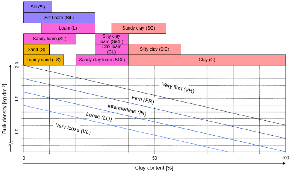
8.4.36 Soil organic carbon (C_org) (m)

Estimation of the content (*)

Report the estimated organic carbon content. It is based on the Munsell value, moist, and the texture. If chroma is 3.5 - 6, use value 0.5 higher (e.g. if you reported a Munsell colour of 10YR 3/4, use a value of 3.5 for estimating soil organic carbon). If chroma is > 6, use value 1 higher.

Caution: The Munsell value is also influenced by parent material, carbonates and redox conditions.

Table 8.84: Estimation of organic carbon contents in a moist sample, Blume et al. (2010), modified

Munsell value	Organic carbon content (%), depending on soil texture class
	S	LS, SL, L	SiL, Si, SiCL, CL, SCL, SC, SiC, C
≥ 6	< 0.2	< 0.2	< 0.2
5.5	< 0.2	< 0.2	0.2 - < 0.5
5	0.2 - < 0.5	0.2 - < 0.5	0.2 - < 0.5
4.5	0.2 - < 0.5	0.2 - < 0.5	0.2 - < 0.5
4	0.2 - < 0.5	0.2 - < 0.5	0.2 - < 1.0
3.5	0.2 - < 1.0	0.5 - < 1.0	0.5 - < 2.5
3	0.5 - < 2.5	1.0 - < 2.5	1.0 - < 5.0
2.5	1.0 - < 5.0	≥ 2.5	≥ 2.5
≤ 2	≥ 2.5

Natural accumulations of organic matter

This Chapter refers to accumulations of organic matter in form of discrete bodies. They have usually a lower value than the surrounding material. Report here all accumulations that are natural or that are a side effect of human activities. For additions of artefacts see Chapter 8.4.8 and of human-transported material see Chapter 8.4.39. If black carbon is purposefully made by humans, it is considered to be an artefact. Organic matter accumulations due to animal activity are reported twice, once here and once in Chapter 8.4.38.

Table 8.85: Types of accumulation of organic matter

Type	Code
Filled earthworm burrows	BU
Filled krotowinas	KR
Organic matter coatings at surfaces of soil aggregates and biopore walls (no visible other material in the coatings)	CO
Black carbon (e.g. charcoal, partly charred particles, soot))	BC
No visible accumulation of organic matter	NO

Report up to three types, the dominant one first, and report the percentage (by exposed area) for each type separately. Black carbon has to be additionally reported as percentage of the exposed area (related to the fine earth plus black carbon of any size).

8.4.37 Roots (o, m)

Count the number of roots per dm², separately for the two diameter classes, and report the abundance classes.

Table 8.86: Abundance of roots, FAO (2006), Table 80

Number ≤ 2 mm	Number > 2 mm	Abundance class	Code
0	0	None	N
1 - 5	1 - 2	Very few	V
6 - 10	3 - 5	Few	F
11 - 20	6 - 10	Common	C
21 - 50	11 - 20	Many	M
> 50	> 20	Abundance	A

8.4.38 Results of animal activity (o, m)

Report the animal activity that has visibly changed the features of the layer. If applicable, report up to 5 types, the dominant one first. Report the percentage (by exposed area), separately for mammal activity, bird activity, worm activity, insect activity and unspecified activity.

Table 8.87: Types of animal activity, FAO (2006), Table 82, modified

Type	Code
Mammal activity
Open large burrows	MO
Infilled large burrows (krotovinas)	MI
Bird activity
Bones, feathers, sorted gravel of similar size	BA
Worm activity
Earthworm channels	WE
Worm casts	WC
Insect activity
Termite channels and nests	IT
Ant channels and nests	IA
Other insect activity	IO
Burrows (unspecified)	BU
No visible results of animal activity	NO

8.4.39 Human alterations (o, m)

Additions of human-transported natural material

Natural material is any material not meeting the criteria of artefacts (see Chapter 8.4.8). Report the percentage (by volume, related to the whole soil), which may range from very little up to 100%, for each addition separately. If more than one occurs, report up to three, the dominant one first. For mineral additions ≤ 2 mm, report additionally, if possible, the texture class (see Chapter 8.4.9), the carbonate content (see Chapter 8.4.25) and the C_org content (see Chapter 8.4.36).

Table 8.88: Artificial additions of natural material

Material	Code
Organic	OR
Mineral, > 2 mm	ML
Mineral, ≤ 2 mm	MS
No additions	NO

In-situ alterations

Report in-situ alterations. If more than one applies, report up to two, the dominant one first.

Table 8.89: In-situ alterations

Type	Code
Ploughing, annually	PA
Ploughing, at least once every 5 years	PO
Ploughing in the past, not ploughed since > 5 years	PP
Ploughing, unspecified	PU
Remodelled (e.g. single ploughing)	RM
Loosening	LO
Compaction, other than a plough pan	CP
Structure deterioration, other than by ploughing or remodelling	SD
Other	OT
No in-situ alteration	NO

Soil aggregate formation after additions or after in-situ alterations

Adding or mixing may combine materials richer and poorer in C_org. A new granular structure may form combining the two. Report, to which extent this process has happened. Use a hand lens.

Table 8.90: Aggregate formation after additions or after in-situ alterations

Criterion	Code
New granular structure present throughout the layer	T
New granular structure present in places, but in other places the added or mixed materials and the previously present materials lie isolated from each other	P
No new granular structure present	N

8.4.40 Parent material (m)

Report the parent material. Use the help of a geological map.

Table 8.91: Types of parent material, FAO (2006), Table 12, modified

Major class	Group	Code	Type	Code
Igneous Rock	Felsic igneous	IF	Granite	IF1
			Quartz-diorite	IF2
			Grano-diorite	IF3
			Diorite	IF4
			Rhyolite	IF5
	Intermediate igneous	II	Andesite, trachyte, phonolite	II1
			Diorite-syenite	II2
	Mafic igneous	IM	Gabbro	IM1
			Basalt	IM2
			Dolerite	IM3
	Ultramafic igneous	IU	Peridotite	IU1
			Pyroxenite	IU2
			Ilmenite, magnetite, ironstone, serpentinite	IU3
	Pyroclastic	IP	Tuff, tuffite	IP1
			Volcanic scoria/breccia	IP2
			Volcanic ash	IP3
			Ignimbrite	IP4
Metamorphic rock	Felsic metamorphic	MF	Quartzite	MF1
			Gneiss, migmatite	MF2
			Slate, phyllite (pelitic rocks)	MF3
			Schist	MF4
	Mafic metamorphic	MM	Slate, phyllite (pelitic rocks	MM1
			(Green)schist	MM2
			Gneiss rich in Fe-Mg minerals	MM3
			Metamorphic limestone (marble)	MM4
			Amphibolite	MM5
			Eclogit	MM6
	Ultramafic metamorphic	MU	Serpentinite, greenstone	MU1
Sedimentary rock (consolidated)	Clastic sediments	SC	Conglomerate, breccia	SC1
			Sandstone, greywacke, arkose	SC2
			Silt-, mud-, claystone	SC3
			Shale	SC4
			Ironstone	SC5
	Carbonatic, organic	SO	Limestone, other carbonate rock	SO1
			Marl and other mixtures	SO2
			Coals, bitumen and related rocks	SO3
	Evaporites	SE	Anhydrite, gypsum	SE1
			Halite	SE2
Sedimentary rock (unconsolidated)	Weathered residuum	UR	Bauxite, laterite	UR1
	Fluvial	UF	Sand and gravel	UF1
			Clay, silt and loam	UF2
	Lacustrine	UL	Sand	UL1
			Silt and clay, < 20% CaCO3 equivalent, little or no diatoms	UL2
			Silt and clay, < 20% CaCO3 equivalent, many diatoms	UL3
			Silt and clay, ≥ 20% CaCO3 equivalent (marl)	UL4
	Marine, estuarine	UM	Sand	UM1
			Clay and silt	UM2
	Colluvial	UC	Slope deposits	UC1
			Lahar	UC2
			Deposit of soil material	UC3
	Aeolian	UE	Loess	UE1
			Sand	UE2
	Glacial	UG	Moraine	UG1
			Glacio-fluvial sand	UG2
			Glacio-fluvial gravel	UG3
	Cryogenic	UK	Periglacial rock debris	UK1
			Periglacial solifluction layer	UK2
	Organic	UO	Rainwater-fed peat (bog)	UO1
			Groundwater-fed peat (fen)	UO2
			Lacustrine (organic limnic sediments)	UO3
	Anthropogenic/ technogenic	UA	Redeposited natural material	UA1
			Industrial/artisanal deposits	UA2
	Unspecified deposits	UU	Clay	UU1
			Loam and silt	UU2
			Sand	UU3
			Gravelly sand	UU4
			Gravel, broken rock	UU5

If the type is unknown, just report the group. Note: the old terms ‘acid’ and ‘basic’ rocks were replaced by ‘felsic’ and ‘mafic’.

8.4.41 Degree of decomposition in organic layers and presence of dead plant residues (o) (*)

Degree of decomposition

This Chapter refers to the transformation of visible plant tissues into visibly homogeneous organic matter. Rub the soil material and report the percentage of visible plant tissues (by volume, related to the fine earth plus all dead plant residues).

Subdivisions of the Oa horizon

If an Oa horizon (see Annex 3, Chapter 10.2) is present, report its subdivisions.

Table 8.92: Subdivisions of the Oa horizon

Criterion	Type	Code
Breaks into longitudinal pieces with sharp edges	Sharp-edged	SE
Breaks into longitudinal pieces with unsharp edges	Compact	CO
Breaks into crumbly pieces or breaks powdery	Crumbly	CR

Dead natural plant residues

This Chapter refers to dead natural plant residues of any length and a diameter ≥ 5 mm. For treated plant residues, see artefacts (see Chapter 8.4.8). Report up to two types of plant remnants, the dominant one first, and give the percentage (by volume, related to the fine earth plus all dead plant residues) for each type separately.

Table 8.93: Dead residues of specific plants

Type of plant residues	Code
Wood	W
Moss fibres	S
Other plants	O
No dead plant residues	N

8.5 Sampling

We describe here the sampling of the terrestrial organic surface layers and the conventional and volumetric sampling of mineral layers, all for the standard analyses described in Annex 2 (Chapter 9). Sampling of other layers requires special techniques that are not described here.

8.5.1 Preparation of sampling bags

Use strong, moisture-resistant bags (transparent, if possible) for sampling. Write the sampling details twice: once on the bag and once on a piece of paper to be put into the bag. If you want to transfer sampling rings to the laboratory, write the sampling details on the ring. Always use a permanent marker.

Write down the following details:

• Profile name
• Conventional (C) / Volumetric (V)
• Layer upper and lower depth
• Layer designation (see Annex 3, Chapter 10).

Example: Gombori Pass 1 - V - 0-10 cm - Ah.

Make sure to seal the bags after filling in the sample.

8.5.2 Sampling of organic layers

Generally, the fine earth plus all dead plant residues are sampled. For the decision if a layer consists of organic material, the organic carbon is measured in a sample containing the fine earth plus the dead plant residues of any length and a diameter ≤ 5 mm (excluding artefacts).

For sampling the terrestrial organic surface layers, use a quadratic steel frame, for instance with 30 cm side length. Use a rubber hammer to drive the frame through the organic surface layers and a few centimetres into the mineral soil. The frame must enter the soil evenly, do not drive in one side first and then the other. Collect the organic surface material manually, sample the litter layer and every O horizon separately. Be very careful to sample all organic surface layers but no mineral layers.

8.5.3 Conventional sampling of mineral layers

Use a scraper to sample every layer separately and along its entire height and width. Start with the lowest layer. Make sure that you only sample one layer at a time, avoid that material from one layer falls into the other.

8.5.4 Volumetric sampling of mineral layers

At the soil surface, determine an area large enough for the appropriate number of sampling rings (e.g. 3 rings). The area must be adjacent to the profile wall and close to the measuring tape. In this area, remove the organic surface layers and start sampling layer by layer from top to down. The thickness of a mineral layer may be larger or smaller than the height of a sampling ring or it may be equal (Figure 8.21).

Figure 8.21: Volumetric sampling

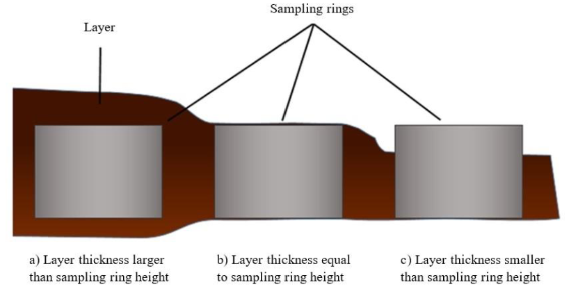
1. If the thickness of the layer is larger, subtract the height of the sampling ring from the layer thickness and divide the difference by 2. This result equals the thickness of soil material that has to be removed starting from the upper layer boundary.
2. If the thickness of the layer is equal, it is very important that the surface is plane.
3. If the thickness of the layer is smaller, you will need the thickness of the layer in relation to the height of the sampling ring for calculating the sampled volume.

For each layer, form a plane surface. If the soil is dryer than field capacity, moisten the surface slowly with water from a spray bottle. Wait until the soil is moist, avoid a water surplus. Then drive in the sampling rings slowly and completely but avoid compacting soil material. For driving in the sampling rings, use a hammer and a piece of wood. The piece should be made of durable wood and have plane surfaces at the top and the bottom. It should be just large enough to cover one sampling ring. If the ring does not move in without deforming, stop driving it in. Try to find a better position.

To take out the rings, penetrate the soil with a spatula just beneath the ring and take it out. If the soil is hard to penetrate, you may use a knife with a serrated blade (bread knife). When necessary, cut roots off. When taking the rings out, make sure that no soil material is lost from inside the rings. Place a cap on the top side and turn the ring upside down. Now make the bottom surface plane and place another cap.

If you want to do further physical analyses, transfer the ring to the laboratory. If the layer thickness is smaller than the height of the ring (case c), fill up the volume with a resin. If you just want to determine the soil mass, you may empty the soil material from the ring into the designated bag and reuse the ring.

To determine the soil mass of a sample of a certain volume, you may also use coated clods (see Annex 2, Chapter 9.5).

Blum, Winfried E. H., Peter Schad, and Stephen Nortcliff. 2018. Essentials of Soil Science: Soil Formation, Functions, Use and Classification (World Reference Base, WRB). Borntraeger Science Publishers. https://www.schweizerbart.de/publications/detail/isbn/9783443010904.

Blume, Hans-Peter, Karl Stahr, and Peter Leinweber. 2010. Bodenkundliches Praktikum: Eine Einführung in Pedologisches Arbeiten Für Ökologen, Insbesondere Land- Und Forstwirte, Und Für Geowissenschaftler. 3rd ed. Springer. https://doi.org/10.1007/978-3-8274-2733-5.

DVWK, ed. 1995. Bodenkundliche Untersuchungen Im Felde Zur Ermittlung von Kennwerten Zur Standortcharakterisierung: Teil i: Ansprache Der Böden. DVWK-Regeln Zur Wasserwirtschaft. Wirtschafts- und Verlagsgesellschaft Gas und Wasser.

Fieldes, Morice, and K. W. Perrott. 1966. “The Nature of Allophane in Soils, Part 3 - Rapid Field and Laboratory Test for Allophane.” New Zealand Journal of Science 9: 623–29. https://www.google.co.nz/books/edition/The_Nature_of_Allophane_in_Soils/3UD9cQAACAAJ?hl=en.

International Organization for Standardization. 2015. Soil Quality — Determination of Particle Size Distribution in Mineral Soil Material — Method by Sieving and Sedimentation. ISO 11277:2009. 2nd ed. https://www.iso.org/standard/54151.html.

Köppen, Wladimir Peter. 1936. Das Geographische System Der Klimat (the Geographical System of the Climate). Handbuch Der Klimatologie. Gebrüder Borntraeger. https://commons.wikimedia.org/wiki/File:Das_geographische_System_der_Klimate_(1936).pdf.

National Committee On Soil And Terrain. 2009. Australian Soil and Land Survey Field Handbook. 3rd ed. Australian Soil and Land Survey Handbooks. CSIRO Publishing. https://www.publish.csiro.au/book/5230/.

Natural England. 2008. Soil Texture. TIN037. Natural England. http://publications.naturalengland.org.uk/publication/32016.

Prietzel, Jörg, and Martin Wiesmeier. 2019. “A Concept to Optimize the Accuracy of Soil Surface Area and SOC Stock Quantification in Mountainous Landscapes.” Geoderma 356 (December): 113922. https://doi.org/10.1016/j.geoderma.2019.113922.

Schoeneberger, P. J., D. A. Wysocki, E. C. Benham, and Soil Survey Staff. 2012. Field Book for Describing and Sampling Soils, Version 3.0. Natural Resources Conservation Service, National Soil Survey Center. https://www.nrcs.usda.gov/sites/default/files/2022-09/field-book.pdf.

Schultz, Jürgen. 2005. The Ecozones of the World: The Ecological Divisions of the Geosphere. 2nd ed. Springer. https://doi.org/10.1007/3-540-28527-X.

Soil Science Division Staff. 2017. Soil Survey Manual. 3rd ed. Agriculture Handbook. United States Department of Agriculture. https://www.nrcs.usda.gov/wps/portal/nrcs/detail/soils/scientists/?cid=nrcs142p2_054262.

Thien, Steve J. 1979. “A Flow Diagram for Teaching Texture-by-Feel Analysis.” Journal of Agronomic Education 8 (1): 54–55. https://doi.org/10.2134/jae.1979.0054.

UN-FAO. 2006. Guidelines for Soil Description. 4th ed. UN-FAO. http://www.fao.org/3/a0541e/a0541e.pdf.